FE Part Wizard
To launch the FE Part creation wizard:
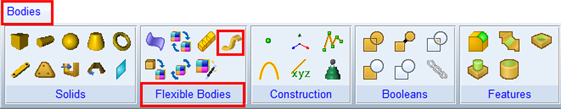
1. Click the Bodies tab on the Adams View ribbon.
2. From the Flexible Bodies container, click the icon for Create FE Part.
3. This wizard may also be accessed by modifying an existing FE Part.
4. Modify wizard for preloaded FE Part having following entries to modify, other than that all entries are disabled. Entries to modify as below:
■Damping Ratio (Stiffness), Damping Ratio (Mass), Location, Orientation on Formulation page
■Define By (disabled and set to “Coordinates”), Preload File on Centerline Page
■Faceting, External Geometry, Datum Node and Contour Plots on Nodes Page
For the option: | Value Type | Do the following: |
|---|---|---|
Page | Formulation | |
Name | New FE Part | If desired, change the default name assigned to the new FE Part type. |
Material | Material | Enter the type of material to be used for the FE Part properties. |
Beam Type | String | Specify the specific type of FE Part to be modelled: ■3D Beam: A three-dimensional fully geometrically nonlinear representation useful for beam-like structures. Accounts for stretching, shearing, bending, and torsion. ■2D Beam XY: A two-dimensional geometrically nonlinear representation useful for beam-like structures whereby the centerline of the beam can be assumed constrained to a plane parallel to the model's global XY plane. 2D Beam can stretch or bend in plane. 2D Beam will solve faster than the 3D Beam. ■2D Beam YZ: A two-dimensional geometrically nonlinear representation useful for beam-like structures whereby the centerline of the beam can be assumed constrained to a plane parallel to the model's global YZ plane. 2D Beam can stretch or bend in plane. 2D Beam will solve faster than the 3D Beam. ■2D Beam ZX: A two-dimensional geometrically nonlinear representation useful for beam-like structures whereby the centerline of the beam can be assumed constrained to a plane parallel to the model's global ZX plane. 2D Beam can stretch or bend in plane. 2D Beam will solve faster than the 3D Beam. |
Damping Ratio (Stiffness) or Visco-elastic damping coefficient ck | Real | Specify the fraction of the stiffness matrix that contributes to the damping matrix for this element. The elastic potential energy of the FE_Part can be expressed as: 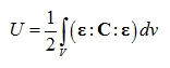 where: ■  is the strain tensor is the strain tensor■C is the constitutive tensor Hence the variation of the elastic potential energy is: 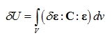 The FE_Part is usually a conservative system, and the total energy of the system is conserved if there is no damping effect. This could cause a problem to the solver, because the high frequency vibrations of FE_Part could make the step size of the solver staying to be intolerable small. In order to damp out the higher frequencies, the variation of the elastic potential energy in Adams FE_Part is expressed as: 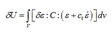 This works very well to damp out the higher frequencies, and have very little effect on the lower frequency motions. It is found that the coefficient ck is very effective in speeding up the simulation, and has little influence on the results if it is set to be small. To learn more about FE Part Damping Ratio (Stiffness), see CRATIOK. |
Damping Ratio (Mass) or Viscous damping coefficient cm | Real | Specify the fraction of the mass matrix that contributes to the damping matrix for this element. The governing equation of the FE_part can be expressed by: 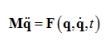 and in Adams, it is usually expressed as follows: 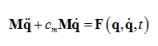 which is similar to the viscous damping in linear vibrations. It is found that cm does not work as good as ck in FE_Part, and it is usually set to be 0 by default. To learn more about FE Part Damping Ratio (Stiffness), see CRATIOM. |
Location | Real,Real,Real | Enter the Cartesian x,y,z coordinates to which you want to move the FE PART object to relative to ground. |
Orientation | Real,Real,Real | Enter the body 313 (body-fixed z, x, z) euler angles to which you want to rotate the FE PART object to relative to ground. |
Page | Centerline | |
Define By | String | Specify the method to be used for centerline definition. ■Curve ■Line from 2 Points |
If "Line from 2 Points" is selected: | ||
Start Point | Existing marker/hard_point | Specify the marker/hard_point that defines start of the FE Part. |
End Point | Existing marker/hard_point | Specify the marker/hard_point that defines end of the FE Part. |
If "Curve" is selected: | ||
Curve | Existing bspline | Specify the geometry (bspline) valid for centerline definition. Note: An FE Part may not close on itself. When selecting a closed curve for the centerline the FE Part will behave as if there is a thin gap between the start and end of the structure. The selected reference curve is hidden automatically after FE part's creation so as to make the FE Part's centerline more easily seen. |
If “Coordinates” is selected: | ||
Coordinates | x, y, z coordinates | Specify x, y, z coordinates on Nodes page. |
Preload | Specifies the name of a file containing preloaded conditions information for this fe_part. | |
Initial Velocity | Checked to give initial velocities on fe_part. | |
All Node | Checked to override the initial properties of all nodes on the FE Part even those which had IC’s individually separately specified via script. Unchecked, Aview will only set the FE Part’s initial velocity properties and therefore, any nodes on which an initial velocity property is set will remain unchanged. | |
Translational velocity along | ||
Ground | Select to specify the global reference coordinates system as the system in which the translational velocity vector components will be specified. | |
Marker | Select and enter a marker along whose axes the translational velocity vector components will be specified. | |
X / Y / Z axis | Select the axes in which you want to define velocity and enter the velocity in the text box that appears next to the axes check boxes. Remember, leaving a velocity unset lets Adams View calculate the velocity of the part during an initial conditions simulation, depending on the other forces and constraints acting on the part. It is not the same as setting the initial velocity to zero. | |
Angular velocity about | ||
LPRF | The components can be locally modeled by referring to position locations to part reference (that is, the “local part reference frame”) and then locating the LPRFs with respect to the system/or every PART contains a unique origin, known as the local part reference frame (LPRF) which is used as the reference coordinate system for any point of interest on the PART. | |
Marker | Select and enter a marker about whose axes the translational or angular velocity vector components will be specified. | |
X / Y / Z axis | Select the axes in which you want to define velocity and enter the velocity in the text box that appears next to the axes check boxes. Remember, leaving a velocity unset lets Adams View calculate the velocity of the part during an initial conditions simulation, depending on the other forces and constraints acting on the part. It is not the same as setting the initial velocity to zero. | |
Page | Nodes | |
Nodes Insert/Delete | The delete button in the wizard works in correspondence with the number entered in the Insert/Delete field. This allows you to Insert/Delete multiple rows at a time. For example, if there are 200 rows and you want to Insert/Delete rows from row 50 onwards, then you should select row 50, type “150” in the field and simply press Insert/Delete. | |
Distance (S) | Real | Specify the position along the length of the centerline; 0 is the start and 1 is the end. Details about how the number and location of nodes can influence extruded geometry. |
X, Y, Z | Real | Specify x, y, z coordinates. Note: These coordinates are only available for the Coordinates Method. |
Angle | Real | A node's X-axis will be oriented in the direction of the curve's instantaneous tangent at the node location. Here, for "Angle," specify the rotation about the node's x-axis defining the orientation of the normal and binormal (that is, the nodes y and z axes). If this value is zero Adams View will, by default, orient the node according to the following rules: ■Node's x-axis will be tangent to curve at node's location ■Node's y-axis and z-axis will be perpendicular to each other with no twist angle about x-axis. |
Section | Section | Specify the section object in the Adams View database that will be used to define the cross-sectional properties of the FE Part at the node. Solid geometry creation for the FE Part can also be defined via the section definition. Note: The following section types do not yet support solid geometry creation (only the centerline geometry will be visible and animate): ♦Hollow rectangle ♦Hollow circle ♦Generic cross-sections where the section will end up as a hollow geometry. Only closed polyline sections are allowed. |
Evenly Distribute | Reset all cells in the "Distance (S)" column so as to evenly space the nodes from Start to End. | |
Uniform Angle | Set all Angle cells to match the value in the Start row. | |
Uniform Section | Apply the section defined in the first row to all rows. | |
Sort by Distance (S) | Will sort and rename all nodes so that they are sequentially ordered by their "Distance (S)" values. Note: This will overwrite the names of any manually named nodes. | |
Evenly Rotate | Reset all cells in the "Angle" column so as to evenly rotate the nodes from Start to End between the current values in the Start and End rows. | |
Curve Control Points | On clicking, the nodes table on the Nodes page will be populated with rows corresponding to each of the spline's control points' positions. It will replace all existing nodes/rows prior to this execution. | |
Parameterize | Upon checking this box the FE Part's set of node (both the number of nodes and their locations, in S, along the reference curve) will be defined by the curve control points now and in the future. That is, if the control points are later moved, then the FE Part nodes will automatically move with them (getting new S values). Note how this differs from the "Curve Control Points" button. The "Curve Control Points" button only sets the number and location of the nodes to match the current reference curve's control points. If those points are subsequently modified the FE Part's number of nodes and their S values would remain the same. See Nodes Parameterization for more information. | |
Faceting Tolerance | Control the density of mesh for FE Part beam. Greater the number, denser the mesh of beam. Default: 300.0, Maximum Limit: 5000.0 | |
The Contour Plots and Datum Node available while modifying the FE part. | ||
Contour Plots | Select this checkbox to enable color contour plotting during animation for the FE Part. The Datum Node can be selected only if the Contour Plots checkbox is selected. | |
Datum Node | The color contour plot of "deformation" is defined by the displacement of the geometry vertices relative to its initial displacement from the datum node. By default the datum node is the node at S=0. To use a different FE Part node please select it here. Note that during the simulation the colors will appear differently than in post-processing animation because the entire extent of deformation throughout the simulation is not yet known thus the color scale is can be changing. | |
External Geometry | ■On: External geometry (Shell/Parasolid) can be imported as a geometry for the FE Part. In this case, no geometry will be created for the FE Part based on the referenced section objects. Only the imported geometry will be used. However, the section properties will be used in Adams Solver calculations that determine the deformation and motion of the FE Part. When importing such files the reference marker must belong to the FE Part and be coincident with the node at S=0. As with all FE Parts, the calculation will assume that the cross-section centroid lies on the FE Part centerline. ■Off: Geometry will be created based on section definitions. | |
Preview | Shows the geometry of FE Part based on inputs given for FE Part. | |