Step Four - Simulating the Model
You will simulate your mechanical model and control system by:
Setting the Simulation Parameters
To set the simulation parameters:
1. From the menus on the Simulink window, select Simulation, and then select Model Configuration Parameters.
The Simulation Parameters dialog box appears.
2. Enter the following simulation parameters:
■For Start Time, enter 0.0 seconds.
■For Stop Time, enter 0.25 seconds.
3. Select the Type text box for the Solver options:
■Set the first text box to Variable-step.
■Set the second text box to ode15s (stiff/NDF).
■Accept the default values in the remaining text boxes.
4. Select OK to close the Simulation Parameters dialog box.
Executing the Simulation
To start the simulation:
■Select Simulation -- Start.
After a few moments, a new Adams View window opens and graphically displays the simulation.
If you’re using Windows, a DOS window appears with the current simulation data. If you’re using Linux, the current simulation data scrolls across the MATLAB window.
Adams accepts the control inputs from MATLAB and integrates the Adams model in response to them. At the same time, Adams provides the azimuthal position and rotor velocity information for MATLAB to integrate the Simulink model. This simulation process creates a closed loop in which the control inputs from MATLAB affect the Adams simulation, and the Adams outputs affect the control input levels. See Figure 2 for an illustration of the closed loop simulation process.
Pausing the Simulation
The interactive capabilities of Adams Controls let you pause the simulation in MATLAB and monitor the graphic results in Adams View. Because MATLAB controls the simulation, you must pause the simulation from within MATLAB. You can plot simulation results during pause mode. This feature is only available when animation mode is set to interactive.
To pause the simulation:
1. A time display in the upper left corner of the Adams screen tracks the seconds of the simulation. To pause the simulation, move your cursor to the Simulink window, point to Simulation, and then select Pause.
MATLAB suspends the simulation.
2. Now go back to Adams View. While the simulation is paused, you can change the orientation of the model with the View Orientation tools in the Standard Toolbar. These tools help you to look at the model from different vantage points.

Figure 11 Standard Toolbar
3. Once you have finished reorienting the model, resume the simulation by selecting Simulation, and then Continue, from the toolbar on the Simulink window.
Adams View closes automatically after the simulation finishes.
Plotting from MATLAB
You can plot any of the data generated in MATLAB. In this tutorial, you will plot the ADAMS_uout data that is saved in the adams_sub block. This block is shown in Figure 12.
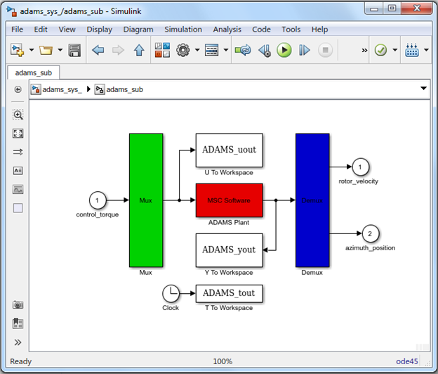
Figure 12 adams_sub Block
To plot from MATLAB:
■At the MATLAB prompt, type in the following command:
>>plot (ADAMS_tout, ADAMS_uout)
The plot window opens and shows the time history of input from MATLAB to Adams. The Figure 13 shows you how the plot should look. Notice that the control torque reaches a peak, and then settles down as the antenna accelerates. As the antenna gets close to its final position, the torque reverses direction to slow down the antenna. The antenna moves past its desired position, and then settles down to the point of zero error. At this point, the torque value is also at zero.
To add labels to your plot:
■At the MATLAB prompt, enter:
>>xlabel(‘Time in seconds’)
>>ylabel(‘Control Torque Input, N-mm’)
>>title(‘Adams Controls Torque Input from MATLAB to Adams’)
>>ylabel(‘Control Torque Input, N-mm’)
>>title(‘Adams Controls Torque Input from MATLAB to Adams’)
The labels appear on the plot.
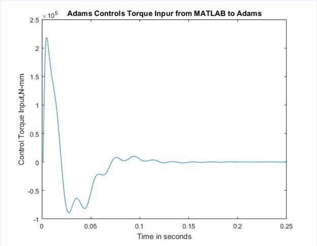
Figure 13 Control Torque Input from MATLAB to Adams
Plotting from Adams View
To plot from Adams View:
1. Start Adams View from your working directory and read in the command file, ant_test.cmd.
2. From the File menu, select Import.
The File Selection dialog box appears.
3. In the File Selection dialog box, select the following:
■For the File Type, select Adams Results File.
■For Files to Read, select Read mytest.res.
■For Model, select main_olt. Be sure to include the model name when you read in results files. Adams View needs to associate the results data with a specific model.
4. Select OK.
The results are loaded. Now, you can plot any data from the cosimulation and play the animation.
5. From the Results tab, select Postprocessor.
Adams View launches Adams PostProcessor, a postprocessing tool that lets you view the results of the simulations you performed (see the Figure 14). Adams PostProcessor has four modes: animation, plotting, reports, and 3D plotting (only available with Adams Vibration data). Note that the page in the plot/animation viewing area can contain up to six viewports to let you compare plots and animations.
Figure 14 Adams PostProcessor Window
6. From the dashboard, set Source to Result Sets.
7. From the Simulation list, select mytest.
8. From the Result Set, select control_torque.
9. From the Component list, select Q.
10. Select Add Curves.
Adams PostProcessor generates the curve.
To add labels to your plot:
1. In the treeview, navigate to the plot and select it.
2. In the Property Editor that appears, perform the following:
■Uncheck Auto Title.
■Set Title to Antenna Azimuth Control Torque in Adams.
■Uncheck Auto Subtitle.
■Set Subtitle to Using Matlab Continuous Controller.
3. Select the vertical axis.
4. In the Property Editor, in the Labels tab, set Label to Control Torque Input (N-mm).
Figure 15 illustrates the torque signal received from the MATLAB controller. The difference between this curve and the one plotted in Figure 13 is because the number of output steps (Adams has fewer outputs).
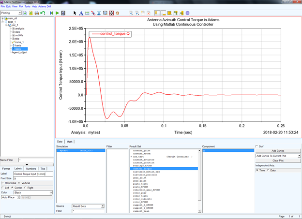
Figure 15 Adams Antenna Joint Peak Torque, Controlled