Step Six - Expose S-Function Parameters to Adams
This section shows how to parameterize your S-Function such that you may be able to automatically create design variables for these parameters in Adams. This section is optional and may be omitted if you do not need to parameterize your S-Function.
Select Parameters
To parameterize an S-Function for Adams, when building the S-Function block using an S-Function target, first create parameters for the Simulink model.
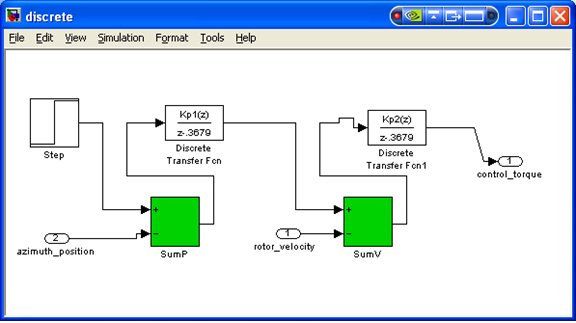
1. Here we will create parameters "Kp1" and "Kp2" to parameterize the gain of the two transfer functions:
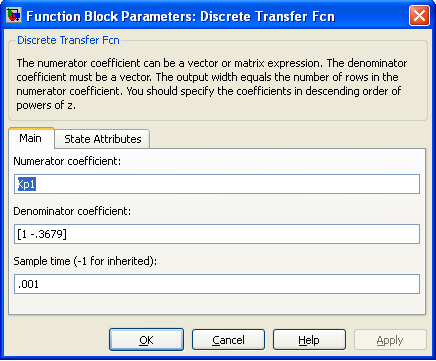
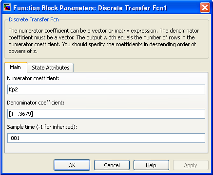
2. Note that you must remove the square brackets [ ] to parameterize this field. The model should now look like the following:
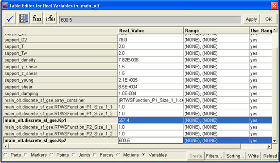
3. Here, we will set the values of the parameters to what they were originally:
>> Kp1=657.4
Kp1 =
657.4000
>> Kp2 = 600.5
Kp2 =
600.5000
Code Generation of Control System
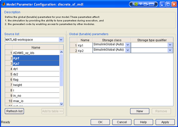
1. Build the S-Function using the S-Function target in RTW and choose the parameters to be Global (tunable) Parameters.
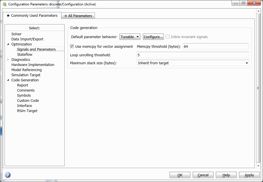
2. Select Code → C/C++ Code → Code Generation Options, select the Optimization → Signals and Parameters tab on the left side, and set the Default parameter behavior to Tunable:
3. Select Configure. This will allow you to select Kp1 and Kp2 add them to the list of Global (tunable) parameters. Do this as below:

4. Choose the Code Generation tab in the Configuration parameters:
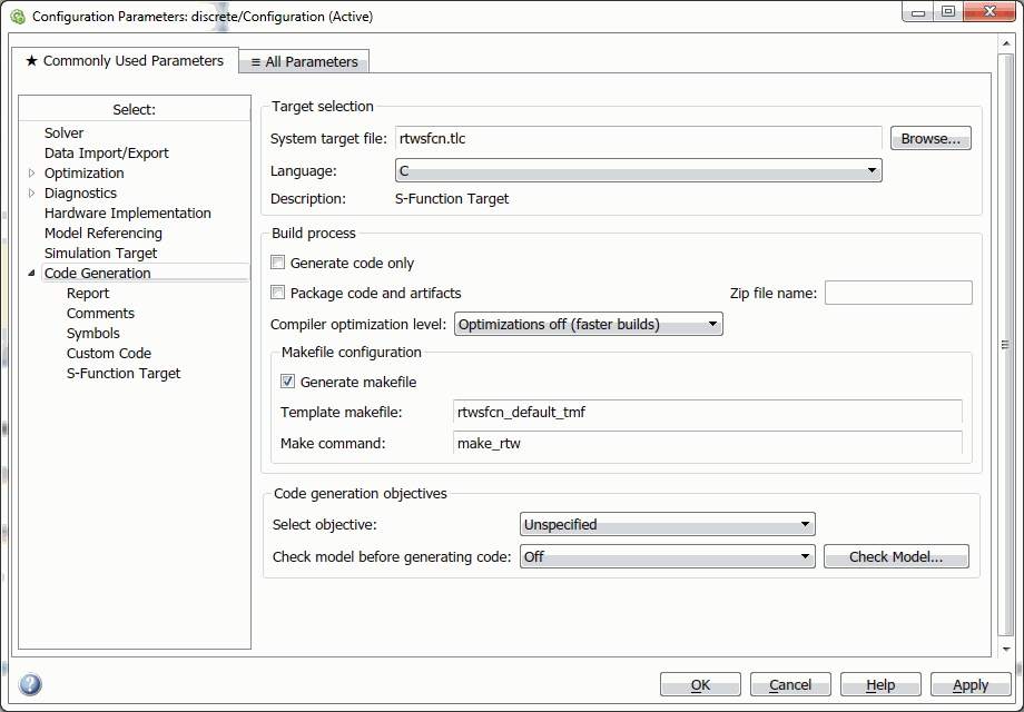
5. Under Configuration Parameters, select the Code Generation tab, and select the S-Function Target for the System Target File.
6. Select Apply and then Build. This should create the file discrete_sf_data.c which will contain the parameters selected:
/* Block parameters (auto storage) */
Parameters_discrete discrete_DefaultParameters = {
6.574E+002,
/* Kp1 : '<Root>/Discrete Transfer Fcn' */
600.5
/* Kp2 : '<Root>/Discrete Transfer Fcn1' */};
7. As in the section, "Step Four - Use S-Function to Create Adams External System Library", create a new model based on your S-Function block, which now has the parameter exposed within it.
In the following steps, you will build the ESL using the Adams Controls-modified RSIM target and again choose the same parameters to be Global (tunable) Parameters.
8. In model with S-Function, select Kp1 and Kp2 as Global (tunable) parameters again:
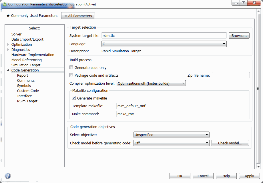
9. Under Configuration Parameters, select the Code Generation tab, and select the Adams Controls-modified RSIM target for the System Target File.
10. Select Apply and then Build. This should create the file discrete_sf_mdl_data.c which will contain the parameters selected (as well as their size (here: 1x1):
/* Block parameters (auto storage) */
Parameters rtP = {
/* RTWSFunction_P1_Size : '<Root>/RTW S-Function' */
{ 1.0, 1.0 }, 6.574E+002,
/* Kp1 : '<Root>/RTW S-Function'*/
/* RTWSFunction_P2_Size : '<Root>/RTW S-Function'*/
{ 1.0, 1.0 }, 600.5
/* Kp2 : '<Root>/RTW S-Function'*/
};
Following the steps in the section, Step Seven - Use the S-Function ESL in Adams Control System Import, you can use Control System Import to load the ESL:
Create GSE from the Simulink Model
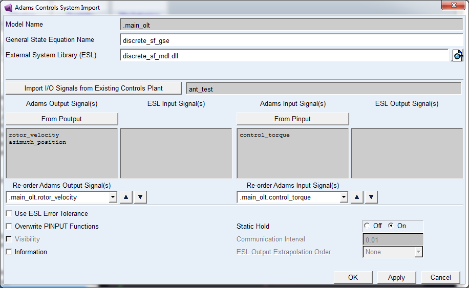
1. After loading the ESL, Adams Controls will show these variables in the Adams Information window:
Object Name : .main_olt.discrete_sf_gse.RTWSFunction_P1_Size_1_1
Object Type : Variable
Parent Type : General_State_Equation
Real Value(s) : 1.0 NO UNITS
Units : no_units
Comment String : None
Object Name : .main_olt.discrete_sf_gse.RTWSFunction_P1_Size_1_2
Object Type : Variable
Parent Type : General_State_Equation
Real Value(s) : 1.0 NO UNITS
Units : no_units
Comment String : None
Object Name : .main_olt.discrete_sf_gse.Kp1
Object Type : Variable
Parent Type : General_State_Equation
Real Value(s) : 657.4 NO UNITS
Units : no_units
Comment String : None
Object Name : .main_olt.discrete_sf_gse.RTWSFunction_P2_Size_1_1
Object Type : Variable
Parent Type : General_State_Equation
Real Value(s) : 1.0 NO UNITS
Units : no_units
Comment String : None
Object Name : .main_olt.discrete_sf_gse.RTWSFunction_P2_Size_1_2
Object Type : Variable
Parent Type : General_State_Equation
Real Value(s) : 1.0 NO UNITS
Units : no_units
Comment String : None
Object Name : .main_olt.discrete_sf_gse.Kp2
Object Type : Variable
Parent Type : General_State_Equation
Real Value(s) : 600.5 NO UNITS
Units : no_units
Comment String : None
Note: | The "size" parameters denote the size of the MATLAB array that stores the parameters. You may ignore these values. |
2. Run a simulation for 0.25 seconds, 250 steps with the default parameter settings.
3. Save this simulation as "baseline".
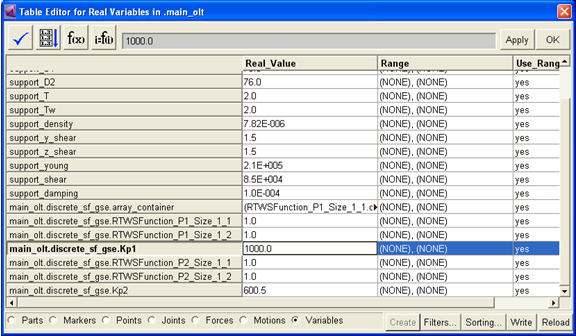
4. Select Tools → Table Editor to modify the parameters from your ESL.
5. Set Kp1 = 1000, as below:
6. Run another simulation for 0.25 seconds, 250 steps with the new parameter settings.
7. Save this simulation as "new".
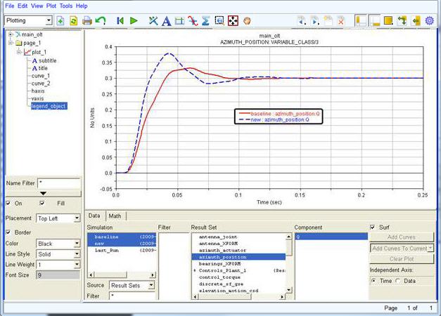
8. Switch to PostProcessor and plot the azimuth position for the baseline vs. new results. You should see something similar to the plot below: