Performing FFT Functions
Learn about Fast fourier transform (FFT) options, how to perform an FFT on a curve, and how to construct a three-dimensional plot.
FFT Representations
Adams PostProcessor contains three methods of representing frequency-domain data:
FFTMAG
FFTMAG (FFT magnitude) determines the magnitude (abs) of the complex value returned from the FFT algorithm. Adams PostProcessor only plots the left spectrum of the frequency data with the frequency on the independent, x-axis, and the magnitude on the dependent, y-axis. The right half of the spectrum is a mirror image of the left half.
Adams PostProcessor scales FFTMAG data by 1/(N/2) where N is the number of time-domain samples. This provides the effect of representing the FFTMAG peak in the magnitude of the time-domain data. The following is an example:

The FFTMAG plot has a peak of 2 at 1 Hz and a peak of 8 at 12 Hz.
Notes: | ■FFTMAG is extremely useful for determining the natural frequencies of structures. ■On the FFT dialog box, there is an option, Detrend Input Data. It removes DC shifts in the data over time. Adams PostProcessor fits a linear regression to the data and subtracts it from the data before performing an FFT. |
FFTPHASE
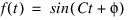
FFTPHASE determines the phase angle of the complex value returned from the standard FFT algorithm. FFTPHASE, at a given frequency, indicates the phase shift of the equivalent sine function represented in the time-domain data. The phase shift of a sinusoidal is phi in the following expression:
PSD (Power Spectral Density)
The signal of any time-dependent model has the same total power in the time domain as in the frequency domain. What is of interest in spectral analysis is the amount of power contained over a frequency interval. A PSD plot represents the distribution of power of a signal among its frequency components. In general, a PSD plot looks like a FFTMAG plot, but on a different scale.
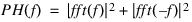
Adams PostProcessor creates a one-sided power spectral density. Therefore, the scaling it uses is:
The PSD option on the FFT dialog box uses the pwelch function in Matlab. The sum of PSD, as computed by pwelch, is equal to the time-integral squared amplitude of the original signal. The pwelch function calculates the PSD using Welch's method:
■The input signal vector x is divided into k overlapping segments according to window and noverlap (or their default values).
■The specified (or default) window is applied to each segment of x.
■An nfft-point FFT is applied to the windowed data.
■The (modified) periodogram of each windowed segment is computed.
■The set of modified periodograms is averaged to form the spectrum estimate S(ej ).
).
).■The resulting spectrum estimate is scaled to compute the power spectral density as S(ej)/F, where F is:
)/F, where F is:■2 pi when you do not supply the sampling frequency.
■fs when you supply the sampling frequency (we use this option in Adams).
The number of segments k that x is divided into is calculated as:
■Eight if you do not specify the window, or if you specify it as the empty vector [].
■k= (m-o)/(l-o) if you specify window as a nonempty vector or a scalar.
In this equation, m is the length of the signal vector x, o is the number of overlapping samples (noverlap), and l is the length of each segment (the window length).
Window Types
The FFT algorithm assumes that the time-domain data is a periodic sample from a continuous, infinite series of data. The beginning and end conditions are, therefore, assumed to match. Window functions are filters that reduce discontinuities from mismatching start and end conditions and ensure periodicity of the FFT.
The window functions are listed below with the equation used to define the window. In the equation, Wj is the window function and N is the number of input samples.
Window functions that closely resemble the unit step input retain the magnitude of the FFT output, but accept minimal discontinuities before the FFT integrity is lost. Likewise, window functions that tend to decrease the accuracy of the peak frequency magnitudes, significantly reduce the negative impact of end condition discontinuities. The application of different window functions depends on the situation and your preference.
Note: | In general, the rectangular window function represents the ideal magnitudes most accurately, but are the most sensitive to discontinuity. The Hanning window function filters the largest discontinuities but represents the ideal magnitudes with the least accuracy. |
Window Functions | Equation Used to Define the Window |
|---|---|
Rectangular | |
Hanning | 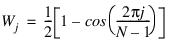 |
Hamming: | 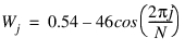 |
Welch | 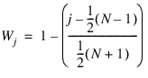 |
Parzen | 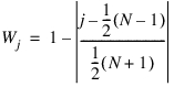 |
Bartlett | For n odd: 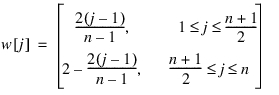 For n even: 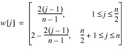 |
Blackman | 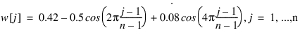 |
Triangular | For n odd: 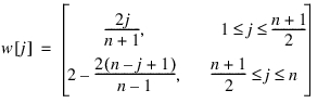 For n even: 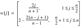 |
Constructing a Two-Dimensional FFT Plot
To create an FFT plot:
1. Select the one or multiple curves on which you want to perform the signal processing.
2. From the Plot menu, select FFT.
The Fast Fourier Transform (FFT) dialog box appears.
3. Select/Browse one or multiple source curves in "Curve Name" field.
4. Set y-axis to Mag, Phase, or PSD.
5. Enter the start and end time on the curve between which you want the signal processing performed.
6. Select the type of window function you want to use. Learn about window types.
7. Specify the number of interpolation points used in fitting the data. The number of points must be a positive integer.
Note: | When you specify the number of points, you are specifying the number of interpolation points used to fit the data in a result set component. Earlier FFT methods required the number of points to be an even power of two (for example, 256, 512, 1024, and so on). With new methods, however, this is no longer necessary. You can select any number of points and the FFT method uses approximation methods to calculate the results. We continue to recommend, however, that the number of points be an even power of two because the results are more precise and the FFT creation is faster. |
8. Select Add Curves to plot multiple curves on same FFT plot window. Continuous pressing of "Add Curves" will superimpose more FFT curves on the same plot.
9. To clear the FFT plot window, select Clear Plot button.
Constructing a Three-Dimensional FFT Plot
You can construct a three-dimensional (3D) Fast fourier transform (FFT) plot by performing signal processing on individual slices of a curve. You define a slice size, and Adams PostProcessor slides this over a range of the curve, overlapping the slices as specified. Each slice of the curve becomes a row in the 3D plot surface.
To create a 3D FFT plot:
1. Select the curve on which you want to perform the signal processing.
2. From the Plot menu, select FFT 3D.
The Fast Fourier Transform (FFT) 3D dialog box appears.
3. Select the type of data to plot in the y-axis: Mag, Phase, or PSD.
4. Enter the start and end time to define the entire range of the curve on which you want signal processing performed.
5. In Time Slice Size, enter the width of the slice on which to perform signal processing, and in Percentage Overlap, enter the percentange amount the slices can overlap.
6. Select the type of window function you want to use.
7. Specify the number of interpolation points used in fitting the data. The number of points must be a positive integer.
8. Select Apply.
Tips on Selecting Points
When you specify the number of points, you are specifying the number of interpolation points used to fit the data in a Result set component. Earlier Fast fourier transform (FFT) methods required the number of points to be an even power of two (for example, 256, 512, 1024, and so on). With new methods, however, this is no longer necessary. You can select any number of points and the FFT method uses approximation methods to calculate the results. We continue to recommend, however, that the number of points be an even power of two because the results are more precise and the FFT creation is faster.
Notes on FFT 3D Plotting
■X values must be in strictly ascending order.
■Frequency option only works with evenly spaced input points. Use interpolate on the curve math toolbar with even output steps turned on to get evenly spaced points.
Constructing a Three-Dimensional FFT Plot for the Order Spectrum
Constructs a three-dimensional (3D) order spectrum plot by performing signal processing on individual slices of a curve with respect to reference rotational velocity. You define a slice size, and Adams PostProcessor slides this over a range of a curve, overlapping the slices as specified. Each slice of the curve becomes a row in the 3D plot surface.
To create a 3D FFT order spectrum plot:
1. Select the curve on which you want to perform the signal processing.
2. From the Plot menu, select FFT 3D.
The Fast Fourier Transform (FFT) 3D dialog box appears.
3. Select the type of plot Order Analysis Order Spectrum from the Plot Type option menu.
4. Select a result set component that represents to them the reference rotational velocity signal defining what constitutes order 1.
5. Select the type of data to plot in the y-axis: Mag, Phase, or PSD.
6. Enter the start and end velocity to define the entire range of the curve on which you want signal processing performed. If left blank at the time of dialog execution, then dialog box execution will use the displayed min and value of rpm from the “Rotational Velocity” result set component.
7. In Velocity Slice Size, enter the width of the slice on which to perform signal processing, and in Percentage Overlap, enter the percentage amount the slices can overlap.
8. Select the type of window function you want to use.
9. Specify the number of interpolation points used in fitting the data. The number of points must be a positive integer.
10. Select Apply.
Note: | It is recommended to use a finer output step sampling rate if better resolution of results is desired at higher orders and rpm. This is because at higher rpm the time window used by the underlying calculation process shrink. |
Constructing a Two-Dimensional Slice of a Three-Dimensional FFT Order Spectrum
You can construct a two-dimensional (2D) slice plot of a three-dimensional (3D) FFT Order spectrum plot by performing a 2D slice at desired order or rpm. There are two options for 2D slices – ‘Amplitude vs. RPM at an order’ or ‘Amplitude vs Order at a RPM’. When ‘Amplitude vs. RPM at an order’ option is selected, you must specify at which order(s) you want to slice the 3D FFT plot. Similarly, when ‘Amplitude vs Order at a RPM’ is selected you must specify at which RPM(s) you want to make the 2D slice.
To create a 2D slice plot:
1. Select the 3D FFT Order analysis plot which you want to use for creating 2D slice plot.
3. Select the type of 2D slice - ‘Amplitude vs. RPM at an order’ or ‘Amplitude vs Order at a RPM’
4. For Amplitude vs. RPM at an order option, enter the order values at which 2D slice(s) should be created and for ‘Amplitude vs Order at a RPM’ enter the RPM values at which 2D slice(s) should be created. Multiple values at a time for order/rpm can be specified for creating multiple 2D slices. If the order/rpm values selected are not available on the 3DFFT plot, an “Out of Bounds” warning message will be issued upon execution.
5. ‘Plot on new page’ will create a new page for 2D slice plot. If the overlay curves option is selected, all the curves will be created in one plot overlaying on one another. If this is not selected, each curve will be plotted as a separate plot.
6. If ‘Plot on same page’ is selected, user can select the plot where the 2D slice plot will be created (all curves will be added to the same plot for this option). If the selected plot is not empty then the current plot will be deleted and new 2D slice plot will be created in place of that plot.
7. Select Apply.