Fast Fourier Transform (FFT) 3D
Edit → Plot → FFT 3D
Constructs a three-dimensional (3D) Fast fourier transform (FFT) plot by performing signal processing on individual slices of a curve. You define a slice size, and Adams PostProcessor slides this over a range of a curve, overlapping the slices as specified. Each slice of the curve becomes a row in the 3D plot surface.
For the option: | Do the following: |
|---|---|
Curve Name | Displays the name of the curve you are plotting. |
Y-Axis | Select one of the following: ■Mag ■PSD |
Z-Axis | Select result set component to be plotted on Z axis. Field execution commands check validity of data in following ways: 1. Data should be in increasing/decreasing order. 2. Data should have evenly spaced points. Time is used by default, when this field is empty. |
Start Time/End Time | Enter the start and end time to define the entire range of the curve on which you want signal processing performed. |
Time Slice Size | Enter the width of a slice of the curve on which to perform signal processing |
Percentage Overlap | Enter the percentage amount the slices can overlap. |
Window Type | Select the type of window you want to use. |
Points/Points (Power of 2) | Select the number of points to be used for the FFT. |
The following option is only available if you selected Mag or Phase. | |
Detrend Input Data | Select if you want to detrend the signal. This subtracts the linear least square fit from the data stream. |
The following options are only available if you selected PSD. | |
Number of Segments/ Segment Length | Enter the number of equal segments into which the signal will be split. Or, you can enter the segment length directly. This is often referred to as the window length. A recommended number of segments is 8, with 50% overlap (see Overlap Points) between segments. |
Overlap Points | Enter the number of overlaps, which indicates how many signal samples are used. With a 50% segment overlap and 8 segments as a recommendation, this number would be Points (Power of 2) / (8*2). |
3D FFT Plotting via the Plot Configuration File
Exporting .plt file for 3D FFT plots.
3D FFT Plots can be saved in a plot configuration file (.plt) like 2D XY plots. See Plot Configuration Files for more information.
Format
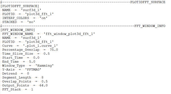
Example illustrating the format of the plot configuration file content when exporting a 3D FFT Plot are shown below. FFT_WINDOW_INFO contains the information about the parameters and the reference plot (curve) used for 3DFFT creation.
3DFFT plots must be exported along with the page containing the reference curve plot. If the reference curve plot is deleted or not included in the exported .plt file, the recreation of 3D FFT plot on importing the exported .plt file may result in errors.
The following warning will be shown if the reference curve plot is not found while exporting 3DFFT plot:

The following warning will be shown if the page with the reference curve plot is available, but not included while exporting 3DFFT plot:

Importing .plt Files with 3D FFT Plots
While importing a plot configuration file (.plt) containing 3D FFT Plots, reference curve plot page will be imported first and the 3DFFT plot will be created based on reference curve and the information from FFT_WINDOW_INFO block of .plt file. If the pages and plots are already present in the PPT window, the pages and plots from .plt file can be renamed automatically, similar to plot curves and 2D FFT plots.
If no reference curve information is present in the .plt file and a plot with the same name is already available in the PPT window, the available plot will be considered as reference curve and the 3D FFT plot will be created.
If no reference curve information is present in the .plt file and no reference curve is available in the PPT window, a warning will be shown and 3D FFT plot will not be created.