Filtering Curve Data
You can filter curve data to eliminate noise on time signals or to emphasize a specific frequency content of a time signal. Adams PostProcessor supports two different types of filters:
■Butterworth filter - butter() in MATLAB developed by The MathWorks, Inc.
■Transfer function - A filter you define by directly specifying the coefficients of a transfer function.
Once you create a filter, you can apply it to any curve.
Learn more about the filters and how to create and apply them:
About Filtering Methods
Adams PostProcessor provides two filtering methods for Fast fourier transform (FFT):
■Analog filtering - The numerical procedure for analog filtering is equivalent to:
■Transfer the time signal into frequency domain through FFT.
■Multiply the resulting function by the filter function.
■Perform an inverse FFT.
■Digital filtering - Digital filtering operates directly on the time signal. The filtered signal at a certain time step is a linear combination of previous input and output signals, with the discrete transfer function defining the coefficients.
Creating and Modifying a Filter Function
You use Filter command on the Plot menu to create or modify a filter function. You can create a Butterworth filter or a transfer function. For the transfer function, you can define the coefficients manually or by defining a Butterworth filter.
To create or modify a Butterworth function:
1. From the Plot menu, point to Filter, and select either Create or Modify. If you selected Modify, select the name of the filter to modify from the Database Navigator.
Tip: | Shortcut for creating a filter: From the Curve Edit toolbar, select the Filter Curve tool  . Right-click the Filter Name text box, point to filter_function, and then select Create. . Right-click the Filter Name text box, point to filter_function, and then select Create. |
The Create/Modify Filter Function dialog box appears.
2. If you are creating a filter, in the Filter Name text box, enter the name you want to assign to the filter function.
3. Select Butterworth Filter.
4. Set the filter type, order, and frequency of cutoff.
5. Select OK.
To create a filter based on a transfer function:
1. From the Plot menu, point to Filter, and select either Create or Modify. If you selected Modify, select the name of the filter to modify from the Database Navigator.
Tip: | Shortcut for creating a filter: From the Curve Edit toolbar, select the Filter Curve tool  . Right-click the Filter Name text box, point to filter_function, and then select Create. . Right-click the Filter Name text box, point to filter_function, and then select Create. |
The Create/Modify Filter Function dialog box appears.
2. If you are creating a filter function, in the Filter Name text box, enter the name you want assigned to the filter function.
3. Select Transfer function.
4. Select a filtering method.
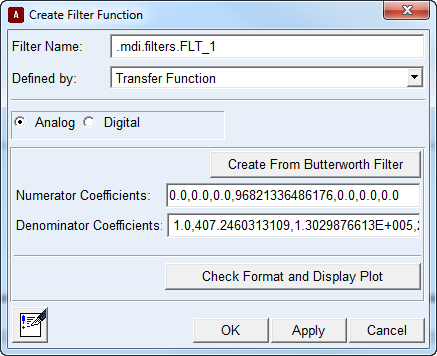
5. Enter the numerator and denominator coefficients as explained in the table below. You can enter the coefficients manually or use a Butterworth filter to define them.
6. To check the format and plot the filter's gain and phase, select Check Format and Display Plot.
If you have not defined the filter correctly, an error message appears. If you've defined the filter correctly, a plot appears in which you can switch between the filter's gain and phase plots and change scales.
7. To associate comments with the filter function, select the Comments tool  , and then enter the comments.
, and then enter the comments. 8. Select OK.
Options for Entering Coefficients
To enter the coefficients: | Do the following: |
|---|---|
Manually | Enter the numerator and denominator coefficients. See Create/Modify Filter Function dialog box help for more information. |
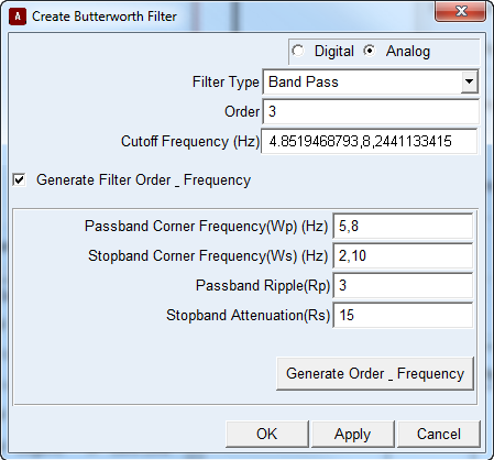
Using a Butterworth filter | 1. Select Create from Butterworth Filter. See Create Butterworth Filter dialog box help for more information. 2. Do one of the following: ■To specify the order and scaled cutoff frequency values directly, enter them at the top of the dialog box. ■To generate them based on Passband and Stopband options, select the checkbox Generate Filter Order _ Frequency. Set the values that appear in the dialog box, and then select the Generate Order _ Frequency button. 3. Select OK. The transfer function coefficients appear in the Create Filter Function dialog box. |
Applying a Filter Function
To apply the filter you created:
1. Select a curve to filter.
 .
. 3. In the Filter Name text box, enter the name of the filter function.
4. To check if compensation for filter lag should be used, select Zero Phase. (Not available for analog filters.)
Zero-phase digital filtering filters the input data in both forward and reverse directions. The resulting sequence has precisely zero-phase distortion and double the filter order.
5. Select OK.
Example of Defining a Transfer Function from a Butterworth Filter
The following example shows how you can define a transfer function by defining a Butterworth filter. The Butterworth filter that you will create is a Basspand filter, based on specifying two values each for passband and stopband corner frequency.
To define a transfer function from a Butterworth filter:
 .
. 2. Right-click the Filter Name text box, point to filter_function, and then select Create.
The Create/Modify Filter Function dialog box appears.
3. In the Filter Name text box, enter bandpass_filter1.
4. Select Transfer function.
5. Select Analog.
6. Set Filter Type to Band Pass.
7. Select Create from Butterworth Filter.
8. Select the Generate Filter Order _ Frequency checkbox.
9. In the Passband Corner Frequency (WP) (Hz) text box, enter 5,8.
10. In the Stopband Corner Frequency (WS) (Hz) text box, enter 2, 10.
11. Leave the default values for Passband Ripple (3) and Stopband Attenuation (15).
12. Select Generate Order _ Frequency.
Adams PostProcessor loads the appropriate values in the Order and Cutoff Frequency text boxes at the top of the dialog box. See the dialog box below for how the values appear.
To view the response:
1. In the Create Butterworth dialog box, select OK.
The following values appear in the Create Filter Function dialog box for numerator and denominator coefficients.
2. Select Check Format and Display Plot.
3. When the plot appears, set the Min to 0.1 and then select Redraw.
The plot appears as follows:
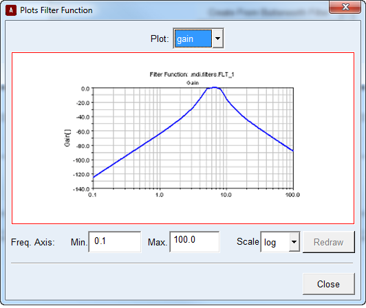
Notice that:
■Between 5 and 8 Hz, the maximum damping is 3dB (specified by the Passband Ripple option).
■At 10 Hz, the damping is 15 dB (specified by the Stopband Attenuation option).
■At 2 Hz, the damping is more than 15 dB; therefore, in this case, it is not a defining factor.