Using the PAC2002 Tire Model
The PAC2002 Magic-Formula tire model has been developed by MSC Software according to Tyre and Vehicle Dynamics by Pacejka [1]. PAC2002 is latest version of a Magic-Formula model available in Adams Tire.
Learn about:
When to Use PAC2002
Magic-Formula (MF) tire models are considered the state-of-the-art for modeling tire-road interaction forces in vehicle dynamics applications. Since 1987, Pacejka and others have published several versions of this type of tire model. The PAC2002 contains the latest developments that have been published in Tyre and Vehicle Dynamics by Pacejka [1].
In general, a MF tire model describes the tire behavior for rather smooth roads (road obstacle wavelengths longer than the tire radius) up to frequencies of 8 Hz. This makes the tire model applicable for all generic vehicle handling and stability simulations, including:
■Steady-state cornering
■Single- or double-lane change
■Braking or power-off in a turn
■Split-mu braking tests
■J-turn or other turning maneuvers
■ABS braking, when stopping distance is important (not for tuning ABS control strategies)
■Other common vehicle dynamics maneuvers
For modeling roll-over of a vehicle, you must pay special attention to the overturning moment characteristics of the tire (Mx) and the loaded radius modeling. The last item may not be sufficiently accurate in this model.
The PAC2002 model has proven to be applicable for car, truck, and aircraft tires with camber (inclination) angles to the road not exceeding 15 degrees.
Originally, Pacejka models have been developed for handling maneuvers at smooth road, as described above. However the PAC2002 has extended functionality that increases the validity towards short road obstacle wavelengths (with use of the 3D Enveloping Contact) and higher frequencies (up to 70 - 80 Hz) by using the tire belt dynamics modeling.
PAC2002 and Previous Magic Formula Models
Compared to previous versions, PAC2002 is backward compatible with all previous versions of PAC2002, MF-Tyre 5.x tire models, and related tire property files.
Modeling of Tire-Road Interaction Forces
For vehicle dynamics applications, an accurate knowledge of tire-road interaction forces is inevitable because the movements of a vehicle primarily depend on the road forces on the tires. These interaction forces depend on both road and tire properties, and the motion of the tire with respect to the road.
In the radial direction, the MF tire models consider the tire to behave as a parallel linear spring and linear damper with one point of contact with the road surface. The contact point is determined by considering the tire and wheel as a rigid disc. In the contact point between the tire and the road, the contact forces in longitudinal and lateral direction strongly depend on the slip between the tire patch elements and the road.
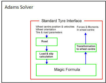
The figure, Input and Output Variables of the Magic Formula Tire Model, presents the input and output vectors of the PAC2002 tire model. The tire model subroutine is linked to the Adams Solver through the Standard Tire Interface (STI) [3]. The input through the STI consists of:
■Position and velocities of the wheel center
■Orientation of the wheel
■Tire model (MF) parameters
■Road parameters
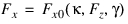
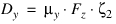
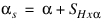
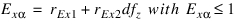
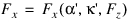
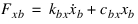
The tire model routine calculates the vertical load and slip quantities based on the position and speed of the wheel with respect to the road. The input for the Magic Formula consists of the wheel load (Fz), the longitudinal and lateral slip  , and inclination angle
  with the road. The output is the forces (Fx, Fy) and moments (Mx, My, Mz) in the contact point between the tire and the road. For calculating these forces, the MF equations use a set of MF parameters, which are derived from tire testing data.
, and inclination angle with the road. The output is the forces (Fx, Fy) and moments (Mx, My, Mz) in the contact point between the tire and the road. For calculating these forces, the MF equations use a set of MF parameters, which are derived from tire testing data.The forces and moments out of the Magic Formula are transferred to the wheel center and returned to Adams Solver through STI.
Input and Output Variables of the Magic Formula Tire Model
Axis Systems and Slip Definitions
Axis Systems
The PAC2002 model is linked to Adams Solver using the TYDEX STI conventions, as described in the TYDEX-Format [2] and the STI [3].
The STI interface between the PAC2002 model and Adams Solver mainly passes information to the tire model in the C-axis coordinate system. In the tire model itself, a conversion is made to the W-axis system because all the modeling of the tire behavior as described in this help assumes to deal with the slip quantities, orientation, forces, and moments in the contact point with the TYDEX W-axis system. Both axis systems have the ISO orientation but have different origin as can be seen in the figure below.
TYDEX C- and W-Axis Systems Used in PAC2002, Source [2]
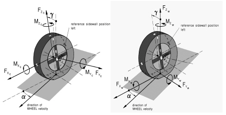
The C-axis system is fixed to the wheel carrier with the longitudinal xc-axis parallel to the road and in the wheel plane (xc-zc-plane). The origin of the C-axis system is the wheel center.
The origin of the W-axis system is the road contact-point defined by the intersection of the wheel plane, the plane through the wheel carrier, and the road tangent plane.
The forces and moments calculated by PAC2002 using the MF equations in this guide are in the W-axis system. A transformation is made in the source code to return the forces and moments through the STI to Adams Solver.
The inclination angle is defined as the angle between the wheel plane and the normal to the road tangent plane (xw-yw-plane).
Units
The units of information transferred through the STI between Adams Solver and PAC2002 are according to the SI unit system. Also, the equations for PAC2002 described in this guide have been developed for use with SI units, although you can easily switch to another unit system in your tire property file. Because of the non-dimensional parameters, only a few parameters have to be changed.
However, the parameters in the tire property file must always be valid for the TYDEX W-axis system (ISO oriented). The basic SI units are listed in the table below (also see Definitions).
SI Units Used in PAC2002
Variable type: | Name: | Abbreviation: | Unit: |
|---|---|---|---|
Angle | Slip angle Inclination angle |   | Radian |
Force | Longitudinal force Lateral force Vertical load | Fx Fy Fz | Newton |
Moment | Overturning moment Rolling resistance moment Self-aligning moment | Mx My Mz | Newton.meter |
Speed | Longitudinal speed Lateral speed Longitudinal slip speed Lateral slip speed | Vx Vy Vsx Vsy | Meters per second |
Rotational speed | Tire rolling speed |  | Radian per second |
Definition of Tire Slip Quantities
The longitudinal slip velocity Vsx in the contact point (W-axis system, see Slip Quantities at Combined Cornering and Braking/Traction) is defined using the longitudinal speed Vx, the wheel rotational velocity  , and the effective rolling radius Re:
, and the effective rolling radius Re: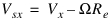 | (1) |
Slip Quantities at Combined Cornering and Braking/Traction
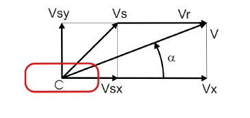
The lateral slip velocity is equal to the lateral speed in the contact point with respect to the road plane:
 | (2) |
The practical slip quantities  (longitudinal slip) and
  (slip angle) are calculated with these slip velocities in the contact point with:
(longitudinal slip) and (slip angle) are calculated with these slip velocities in the contact point with: | (3) |
 | (4) |
The rolling speed Vr is determined using the effective rolling radius Re:
 | (5) |
Turn-slip is one of the two components that form the spin of the tire. Turn-slip  is calculated using the tire yaw velocity
  :
:
is calculated using the tire yaw velocity : | (6) |
The total tire spin  is calculated using:
is calculated using: | (7) |
The total tire spin has contributions of turn-slip and camber.  denotes the camber reduction factor for the camber to become comparable with turn-slip.
denotes the camber reduction factor for the camber to become comparable with turn-slip.Contact Methods and Normal Load Calculation
Contact Methods
The PAC2002 tire model supports all Adams Tire contact methods.
■One Point Follower Contact, used by default for 2D Road, 3D Spline Road, OpenCRG Road and RGR Road.
■3D Equivalent Volume Contact, used by default for 3D Shell Road.
■3D Enveloping Contact, can be used with all road types when the keyword CONTACT_MODEL = '3D_ENVELOPING' is specified in the [MODEL] section of the tire property file.
In vertical direction, the PAC2002 tire is modeled as a parallel spring and damper. The spring deflection and damper velocity are derived with the (effective) road height and plane information supplied by the contact method.
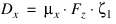
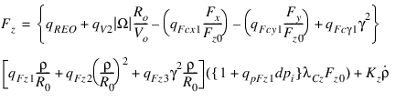
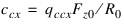
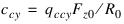
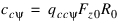
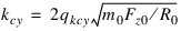
The normal load Fz of the tire is calculated with the tire deflection  as follows:
as follows: | (8) |
Using this formula, the vertical tire stiffness increases due to increasing rotational speed  and decreases by longitudinal and lateral tire forces. If qFz1 and qFz2 are zero, qFz1 will be defined as CzR0/Fz0.
and decreases by longitudinal and lateral tire forces. If qFz1 and qFz2 are zero, qFz1 will be defined as CzR0/Fz0.Parameter qRE0 corrects for possible differences in between the specified unloaded radius (R0) and the measured radius in tire testing.
When you do not provide the coefficients qV2, qFcx, qFcy, qFz1, qFz2 and qFz3 in the tire property file, the normal load calculation is compatible with previous versions of PAC2002, because, in that case, the normal load is calculated using the linear vertical tire stiffness Cz and tire damping Kz according to:
Instead of the linear vertical tire stiffness Cz (= qFz1Fz0/R0), you can define an arbitrary tire deflection - load curve in the tire property file in the section [DEFLECTION_LOAD_CURVE] (see the Example of PAC2002 Tire Property File). If a section called [DEFLECTION_LOAD_CURVE] exists, the load deflection data points with a cubic spline for inter- and extrapolation are used for the calculation of the vertical force of the tire. Note that you must specify Cz in the tire property file, but it does not play any role.
Loaded and Effective Tire Rolling Radius
With the loaded tire radius Rl defined as the distance of the wheel center to the contact point of the tire with the road, the tire deflection can be calculated using the free tire radius R0 and a correction for the tire radius growth due to the rotational tire speed  :
:
:  | (9) |
The effective rolling radius Re (at free rolling of the tire), which is used to calculate the rotational speed of the tire, is defined by:
 | (10) |
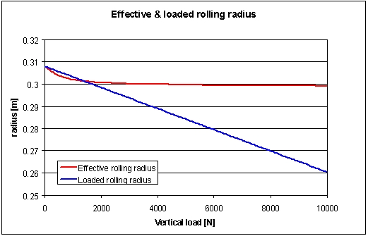
For radial tires, the effective rolling radius is rather independent of load in its load range of operation because of the high stiffness of the tire belt circumference. Only at low loads does the effective tire radius decrease with increasing vertical load due to the tire tread thickness. See the figure below.
Effective Rolling Radius and Longitudinal Slip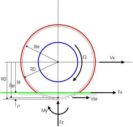
To represent the effective rolling radius Re, a MF-type of equation is used:
 | (11) |
in which  Fz0 is the nominal tire deflection:
Fz0 is the nominal tire deflection: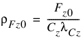 | (12) |
and  is called the dimensionless radial tire deflection, defined by:
is called the dimensionless radial tire deflection, defined by: | (13) |
Example of Loaded and Effective Tire Rolling Radius as Function of Vertical Load
Normal Load and Rolling Radius Parameters
Name: | Name Used in Tire Property File: | Explanation: |
|---|---|---|
Fz0 | FNOMIN | Nominal wheel load |
Ro | UNLOADED_RADIUS | Free tire radius |
BReff | BREFF | Low load stiffness effective rolling radius |
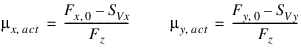
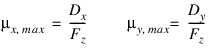
qREO | QREO | Correction factor for measured unloaded radius |
DReff | DREFF | Peak value of effective rolling radius |
FReff | FREFF | High load stiffness effective rolling radius |
Cz | VERTICAL_STIFFNESS | Tire vertical stiffness (if qFz1=0) |
Kz | VERTICAL_DAMPING | Tire vertical damping |
qFz1 | QFZ1 | Tire vertical stiffness coefficient (linear) |
qFz2 | QFZ2 | Tire vertical stiffness coefficient (quadratic) |
qFz3 | QFZ3 | Camber dependency of the tire vertical stiffness |
qFcx1 | QFCX1 | Tire stiffness interaction with Fx |
qFcy1 | QFCY1 | Tire stiffness interaction with Fy |
qFc  1 1 | QFCG1 | Tire stiffness interaction with camber |
qV1 | QV1 | Tire radius growth coefficient |
qV2 | QV2 | Tire stiffness variation coefficient with speed |
Wheel Bottoming
You can optionally supply a wheel-bottoming deflection, that is, a load curve in the tire property file in the [BOTTOMING_CURVE] block. If the deflection of the wheel is so large that the rim will be hit (defined by the BOTTOMING_RADIUS parameter in the [DIMENSION] section of the tire property file), the tire vertical load will be increased according to the load curve defined in this section.
Note that the rim-to-road contact algorithm is a simple penetration method (such as the 2D contact) based on the tire-to-road contact calculation, which is strictly valid for only rather smooth road surfaces (the length of obstacles should have a wavelength longer than the tire circumference). The rim-to-road contact algorithm is not based on the 3D-volume penetration method, but can be used in combination with the 3D Contact, which takes into account the volume penetration of the tire itself. If you omit the [BOTTOMING_CURVE] block from a tire property file, no force due to rim road contact is added to the tire vertical force.
You can choose a BOTTOMING_RADIUS larger than the rim radius to account for the tire's material remaining in between the rim and the road, while you can adjust the bottoming load-deflection curve for the change in stiffness.
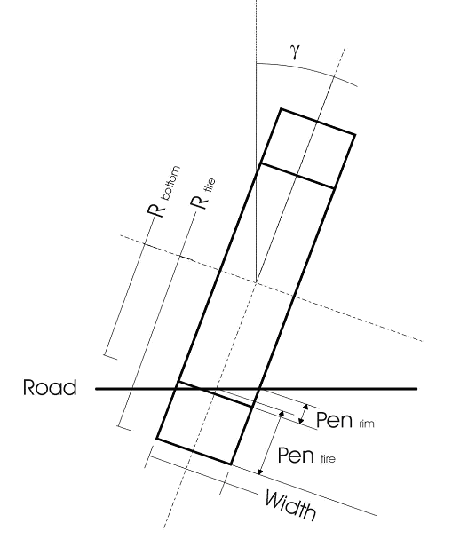
If (Pentire - (Rtire - Rbottom) - ½·width ·| tan(γ) |) < 0, the left or right side of the rim has contact with the road. Then, the rim deflection Penrim can be calculated using:
 = max(0 , ½·width ·| tan(
 ) | ) + Pentire- (Rtire - Rbottom)
 Penrim=  /(2 · width ·| tan(
 ) |)
) |)
/(2 · width ·| tan() |) Srim= ½·width - max(width ,  /| tan(
 ) |)/3
/| tan() |)/3 with Srim, the lateral offset of the force with respect to the wheel plane.
If the full rim has contact with the road, the rim deflection is:
Penrim = Pentire - (Rtire - Rbottom)
Srim = width2 · | tan( ) | · /(12 · Penrim)
) | · /(12 · Penrim) Using the load - deflection curve defined in the [BOTTOMING_CURVE] section of the tire property file, the additional vertical force due to the bottoming is calculated, while Srim multiplied by the sign of the inclination  is used to calculate the contribution of the bottoming force to the overturning moment. Further, the increase of the total wheel load Fz due to the bottoming (Fzrim) will not be taken into account in the calculation for Fx, Fy, My, and Mz. Fzrim will only contribute to the overturning moment Mx using the Fzrim·Srim.
is used to calculate the contribution of the bottoming force to the overturning moment. Further, the increase of the total wheel load Fz due to the bottoming (Fzrim) will not be taken into account in the calculation for Fx, Fy, My, and Mz. Fzrim will only contribute to the overturning moment Mx using the Fzrim·Srim. Note: | Rtire is equal to the unloaded tire radius R0; Pentire is similar to effpen (=  ). ). |
Basics of the Magic Formula in PAC2002
The Magic Formula is a mathematical formula that is capable of describing the basic tire characteristics for the interaction forces between the tire and the road under several steady-state operating conditions. We distinguish:
■Pure cornering slip conditions: cornering with a free rolling tire
■Pure longitudinal slip conditions: braking or driving the tire without cornering
■Combined slip conditions: cornering and longitudinal slip simultaneously
For pure slip conditions, the lateral force Fy as a function of the lateral slip  , respectively, and the longitudinal force Fx as a function of longitudinal slip
  , have a similar shape (see the figure, Characteristic Curves for Fx and Fy Under Pure Slip Conditions). Because of the sine - arctangent combination, the basic Magic Formula equation is capable of describing this shape:
, respectively, and the longitudinal force Fx as a function of longitudinal slip , have a similar shape (see the figure, Characteristic Curves for Fx and Fy Under Pure Slip Conditions). Because of the sine - arctangent combination, the basic Magic Formula equation is capable of describing this shape: | (14) |
where Y(x) is either Fx with x the longitudinal slip  , or Fy and x the lateral slip
  .
.
, or Fy and x the lateral slip .Characteristic Curves for Fx and Fy Under Pure Slip Conditions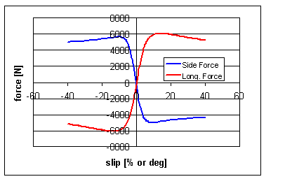
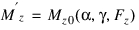
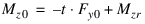
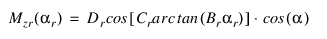
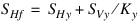
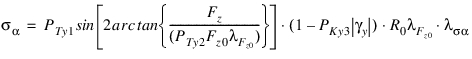
The self-aligning moment Mz is calculated as a product of the lateral force Fy and the pneumatic trail t added with the residual moment Mzr. In fact, the aligning moment is due to the offset of lateral force Fy, called pneumatic trail t, from the contact point. Because the pneumatic trail t as a function of the lateral slip α has a cosine shape, a cosine version the Magic Formula is used:
 | (15) |
in which Y(x) is the pneumatic trail t as function of slip angle  .
.
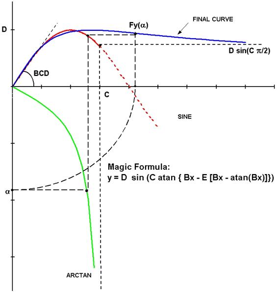
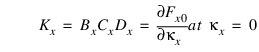
.The figure, The Magic Formula and the Meaning of Its Parameters, illustrates the functionality of the B, C, D, and E factor in the Magic Formula:
■D-factor determines the peak of the characteristic, and is called the peak factor.
■C-factor determines the part used of the sine and, therefore, mainly influences the shape of the curve (shape factor).
■B-factor stretches the curve and is called the stiffness factor.
■E-factor can modify the characteristic around the peak of the curve (curvature factor).
The Magic Formula and the Meaning of Its Parameters
In combined slip conditions, the lateral force Fy will decrease due to longitudinal slip or the opposite, the longitudinal force Fx will decrease due to lateral slip. The forces and moments in combined slip conditions are based on the pure slip characteristics multiplied by the so-called weighing functions. Again, these weighting functions have a cosine-shaped MF equation.
The Magic Formula itself only describes steady-state tire behavior. For transient tire behavior (up to 8 Hz), the MF output is used in a stretched string model that considers tire belt deflections instead of slip velocities to cope with standstill situations (zero speed).
Input Variables
The input variables to the Magic Formula are:
Longitudinal slip |  | [-] |
Slip angle |  | [rad] |
Inclination angle |  | [rad] |
Normal wheel load | Fz | [N] |
Output Variables
Longitudinal force | Fx | [N] |
Lateral force | Fy | [N] |
Overturning couple | Mx | [Nm] |
Rolling resistance moment | My | [Nm] |
Aligning moment | Mz | [Nm] |
The output variables are defined in the W-axis system of TYDEX.
Basic Tire Parameters
All tire model parameters of the model are without dimension. The reference parameters for the model are:
Name | Name used in tire property file | Unit | Explanation |
|---|---|---|---|
Fz0 | FNOMIN | [N] | Nominal (rated) load |
R0 | UNLOADED_RADIUS | [m] | Unloaded tire radius |
pi0 | IP_NOM | [Pa] | Nominal inflation pressure |
pi | IP | [Pa] | Actual inflation pressure |
m0 | TYRE_MASS | [kg] | Tire mass (if belt dynamics is used) |
As a measure for the vertical load, the normalized vertical load increment dfz is used:
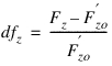 | (16) |
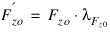
with the possibly adapted nominal load (using the user-scaling factor,  ):
):
):
Similarly the normalized inflation pressure dpi is defined as:
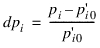 | (17) |
With the user scaling factor for the inflation pressure:

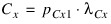
Nomenclature of the Tire Model Parameters
In the subsequent sections, formulas are given with non-dimensional parameters aijk with the following logic:
Tire Model Parameters
Parameter: | Definition: | |
|---|---|---|
a = | p | Force at pure slip |
q | Moment at pure slip | |
r | Force at combined slip | |
s | Moment at combined slip | |
i = | B | Stiffness factor |
C | Shape factor | |
D | Peak value | |
E | Curvature factor | |
K | Slip stiffness = BCD | |
H | Horizontal shift | |
V | Vertical shift | |
s | Moment at combined slip | |
t | Transient tire behavior | |
j = | x | Along the longitudinal axis |
y | Along the lateral axis | |
z | About the vertical axis | |
k = | 1, 2, ... | |
User Scaling Factors
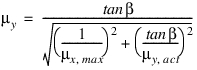
A set of scaling factors is available to easily examine the influence of changing tire properties without the need to change one of the real Magic Formula coefficients. The default value of these factors is 1. You can change the factors in the tire property file. The peak friction scaling factors,  and
and  , are also used for the position-dependent friction in 3D Road Contact and 3D Road. An overview of all scaling factors is shown in the following tables.
and , are also used for the position-dependent friction in 3D Road Contact and 3D Road. An overview of all scaling factors is shown in the following tables.Scaling Factor Coefficients for Pure Slip
Name: | Name used in tire property file: | Explanation: |
|---|---|---|
 Fzo Fzo | LFZO | Scale factor of nominal (rated) load |
 ip ip | LIP | Scale factor of nominal inflation pressure |
 Cz Cz | LCZ | Scale factor of vertical tire stiffness |
 Cx Cx | LCX | Scale factor of Fx shape factor |
 | LMUX | Scale factor of Fx peak friction coefficient |
 Ex Ex | LEX | Scale factor of Fx curvature factor |
 Kx Kx | LKX | Scale factor of Fx slip stiffness |
 Hx Hx | LHX | Scale factor of Fx horizontal shift |
 Vx Vx | LVX | Scale factor of Fx vertical shift |
 | LGAX | Scale factor of inclination for Fx |
 Cy Cy | LCY | Scale factor of Fy shape factor |
 | LMUY | Scale factor of Fy peak friction coefficient |
 Ey Ey | LEY | Scale factor of Fy curvature factor |
 Ky Ky | LKY | Scale factor of Fy cornering stiffness |
 Hy Hy | LHY | Scale factor of Fy horizontal shift |
 Vy Vy | LVY | Scale factor of Fy vertical shift |
 gy gy | LGAY | Scale factor of inclination for Fy |
 | LKG | Scale factor of the camber stiffness  |
 t t | LTR | Scale factor of peak of pneumatic trail |
 Mr Mr | LRES | Scale factor for offset of residual moment |
 | LGAZ | Scale factor of inclination for Mz |
 Mx Mx | LMX | Scale factor of overturning couple |
 VMx VMx | LVMX | Scale factor of Mx vertical shift |
 My My | LMY | Scale factor of rolling resistance moment |
Scaling Factor Coefficients for Combined Slip
Name: | Name used in tire property file: | Explanation: |
|---|---|---|
 xα xα | LXAL | Scale factor of alpha influence on Fx |
 yκ yκ | LYKA | Scale factor of alpha influence on Fy |
 Vyκ Vyκ | LVYKA | Scale factor of kappa-induced Fy |
 | LS | Scale factor of moment arm of Fx |
Scaling Factor Coefficients for Transient Response
Name: | Name used in tire property file: | Explanation: |
|---|---|---|
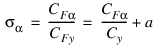
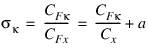
 σκ σκ | LSGKP | Scale factor of relaxation length of Fx |
 σα σα | LSGAL | Scale factor of relaxation length of Fy |
 gyr gyr | LGYR | Scale factor of gyroscopic moment |
Note that the scaling factors change during the simulation according to any user-introduced function. See the next section, Online Scaling of Tire Properties.
Online Scaling of Tire Properties
PAC2002 can provide online scaling of tire properties. For each scaling factor, a variable should be introduced in the Adams .adm dataset. For example:
!lfz0 scaling
! adams_view_name='TR_Front_Tires until wheel_lfz0_var'
VARIABLE/53
, IC = 1
, FUNCTION = 1.0
This lets you change the scaling factor during a simulation as a function of time or any other variable in your model. Therefore, tire properties can change because of inflation pressure, road friction, road temperature, and so on.
You can also use the scaling factors in co-simulations in MATLAB/Simulink.
For more detailed information, see Simcompanion Knowledge Base Article KB8016467.
Steady-State: Magic Formula in PAC2002
Steady-State Pure Slip
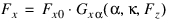
Formulas for the Longitudinal Force at Pure Slip
For the tire rolling on a straight line with no slip angle, the formulas are:
 | (18) |
 | (19) |
 | (20) |
 | (21) |
with following coefficients:
 | (22) |
 | (23) |
 | (24) |
 | (25) |
the longitudinal slip stiffness:
 | (26) |
 | (27) |
 | (28) |
 | (29) |
Longitudinal Force Coefficients at Pure Slip
Name: | Name used in tire property file: | Explanation: |
|---|---|---|
pCx1 | PCX1 | Shape factor Cfx for longitudinal force |
pDx1 | PDX1 | Longitudinal friction Mux at Fznom |
pDx2 | PDX2 | Variation of friction Mux with load |
pDx3 | PDX3 | Variation of friction Mux with inclination |
pEx1 | PEX1 | Longitudinal curvature Efx at Fznom |
pEx2 | PEX2 | Variation of curvature Efx with load |
pEx3 | PEX3 | Variation of curvature Efx with load squared |
pEx4 | PEX4 | Factor in curvature Efx while driving |
pKx1 | PKX1 | Longitudinal slip stiffness Kfx/Fz at Fznom |
pKx2 | PKX2 | Variation of slip stiffness Kfx/Fz with load |
pKx3 | PKX3 | Exponent in slip stiffness Kfx/Fz with load |
pHx1 | PHX1 | Horizontal shift Shx at Fznom |
pHx2 | PHX2 | Variation of shift Shx with load |
pVx1 | PVX1 | Vertical shift Svx/Fz at Fznom |
pVx2 | PVX2 | Variation of shift Svx/Fz with load |
ppx1 | PPX1 | Variation of slip stiffness Kfx/Fz with pressure |
ppx2 | PPX2 | Variation of slip stiffness Kfx/Fz with pressure squared |
ppx3 | PPX3 | Variation of friction Mux with pressure |
ppx4 | PPX4 | Variation of friction Mux with pressure squared |
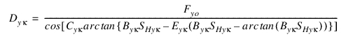
Formulas for the Lateral Force at Pure Slip
 | (30) |
 | (31) |
 | (32) |
The scaled inclination angle:
 | (33) |
with coefficients:
 | (34) |
 | (35) |
 | (36) |
 | (37) |
The cornering stiffness:
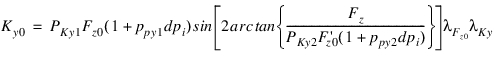 | (38) |
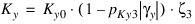 | (39) |
 | (40) |
 | (41) |
 | (42) |
 | (43) |
The camber stiffness is given by:
 | (44) |
Lateral Force Coefficients at Pure Slip
Name: | Name used in tire property file: | Explanation: |
|---|---|---|
pCy1 | PCY1 | Shape factor Cfy for lateral forces |
pDy1 | PDY1 | Lateral friction Muy |
pDy2 | PDY2 | Variation of friction Muy with load |
pDy3 | PDY3 | Variation of friction Muy with squared inclination |
pEy1 | PEY1 | Lateral curvature Efy at Fznom |
pEy2 | PEY2 | Variation of curvature Efy with load |
pEy3 | PEY3 | Inclination dependency of curvature Efy |
pEy4 | PEY4 | Variation of curvature Efy with inclination |
pKy1 | PKY1 | Maximum value of stiffness Kfy/Fznom |
pKy2 | PKY2 | Load at which Kfy reaches maximum value |
pKy3 | PKY3 | Variation of Kfy/Fznom with inclination |
pHy1 | PHY1 | Horizontal shift Shy at Fznom |
pHy2 | PHY2 | Variation of shift Shy with load |
pHy3 | PHY3 | Variation of shift Shy with inclination |
pVy1 | PVY1 | Vertical shift in Svy/Fz at Fznom |
pVy2 | PVY2 | Variation of shift Svy/Fz with load |
pVy3 | PVY3 | Variation of shift Svy/Fz with inclination |
pVy4 | PVY4 | Variation of shift Svy/Fz with inclination and load |
ppy1 | PPY1 | Variation of max. stiffness Kfy/Fznom with pressure |
ppy2 | PPY2 | Variation of load at max. Kfy with pressure |
ppy3 | PPY3 | Variation of friction Muy with pressure |
ppy4 | PPY4 | Variation of friction Muy with pressure squared |
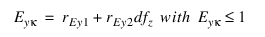
Formulas for the Aligning Moment at Pure Slip
 | (45) |
with the pneumatic trail t:
 | (46) |
 | (47) |
and the residual moment Mzr:
 | (48) |
 | (49) |
 | (50) |
The scaled inclination angle:
 | (51) |
with coefficients:
 | (52) |
 | (53) |
 | (54) |
 | (55) |
 | (56) |
 | (57) |

 | (58) |
An approximation for the aligning moment stiffness reads:
 | (59) |
Aligning Moment Coefficients at Pure Slip
Name: | Name used in tire property file: | Explanation: |
|---|---|---|
qBz1 | QBZ1 | Trail slope factor for trail Bpt at Fznom |
qBz2 | QBZ2 | Variation of slope Bpt with load |
qBz3 | QBZ3 | Variation of slope Bpt with load squared |
qBz4 | QBZ4 | Variation of slope Bpt with inclination |
qBz5 | QBZ5 | Variation of slope Bpt with absolute inclination |
qBz9 | QBZ9 | Slope factor Br of residual moment Mzr |
qBz10 | QBZ10 | Slope factor Br of residual moment Mzr |
qCz1 | QCZ1 | Shape factor Cpt for pneumatic trail |
qDz1 | QDZ1 | Peak trail Dpt = Dpt*(Fz/Fznom*R0) |
qDz2 | QDZ2 | Variation of peak Dpt with load |
qDz3 | QDZ3 | Variation of peak Dpt with inclination |
qDz4 | QDZ4 | Variation of peak Dpt with inclination squared. |
qDz6 | QDZ6 | Peak residual moment Dmr = Dmr/ (Fz*R0) |
qDz7 | QDZ7 | Variation of peak factor Dmr with load |
qDz8 | QDZ8 | Variation of peak factor Dmr with inclination |
qDz9 | QDZ9 | Variation of Dmr with inclination and load |
qEz1 | QEZ1 | Trail curvature Ept at Fznom |
qEz2 | QEZ2 | Variation of curvature Ept with load |
qEz3 | QEZ3 | Variation of curvature Ept with load squared |
qEz4 | QEZ4 | Variation of curvature Ept with sign of Alpha-t |
qEz5 | QEZ5 | Variation of Ept with inclination and sign Alpha-t |
qHz1 | QHZ1 | Trail horizontal shift Sht at Fznom |
qHz2 | QHZ2 | Variation of shift Sht with load |
qHz3 | QHZ3 | Variation of shift Sht with inclination |
qHz4 | QHZ4 | Variation of shift Sht with inclination and load |
qpz1 | QPZ1 | Variation of peak Dt with pressure |
qpz2 | QPZ2 | Variation of peak Dr with pressure |
Turn-slip and Parking
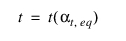
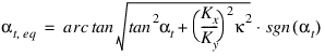
For situations where turn-slip may be neglected and camber remains small, the reduction factors  that appear in the equations for steady-state pure slip, are to be set to 1:
that appear in the equations for steady-state pure slip, are to be set to 1:
For larger values of spin, the reduction factors are given below.
The weighting function  is used to let the longitudinal force diminish with increasing spin, according to:
is used to let the longitudinal force diminish with increasing spin, according to: | (60) |
with:
 | (61) |
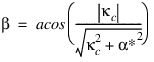
The peak side force reduction factor  reads:
reads: | (62) |
with:
 | (63) |
The cornering stiffness reduction factor  is given by:
is given by: | (64) |
The horizontal shift of the lateral force due to spin is given by:
 | (65) |
The factors are defined by:
 | (66) |
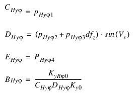
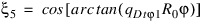
The spin force stiffness KyRϕ0 is related to the camber stiffness Kyy0:
 | (67) |
in which the camber reduction factor is given by:
 | (68) |
The reduction factors  and
and  for the vertical shift of the lateral force are given by:
and for the vertical shift of the lateral force are given by: | (69) |
The reduction factor for the residual moment reads:
 | (70) |
The peak spin torque Dr is given by:
is given by: | (71) |
The maximum value is given by:
 | (72) |
The pneumatic trail reduction factor due to turn slip is given by:
 | (73) |
The moment at vanishing wheel speed at constant turning is given by:
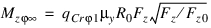 | (74) |
The shape factors are given by:
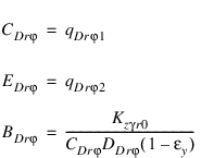 | (75) |
in which:
 | (76) |
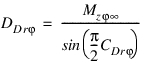
The reduction factor  reads:
reads: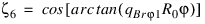 | (77) |
The spin moment at 90º slip angle is given by:
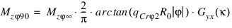 | (78) |
The spin moment at 90º slip angle is multiplied by the weighing function  to account for the action of the longitudinal slip (see steady-state combined slip equations).
to account for the action of the longitudinal slip (see steady-state combined slip equations).The reduction factor  is given by:
is given by: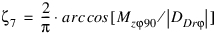 | (79) |
Turn-Slip and Parking Parameters
Name: | Name used in tire property file: | Explanation: |
|---|---|---|
pεγϕ1 | PECP1 | Camber spin reduction factor parameter in camber stiffness. |
pεγϕ2 | PECP2 | Camber spin reduction factor varying with load parameter in camber stiffness. |
pDxϕ1 | PDXP1 | Peak Fx reduction due to spin parameter. |
pDxϕ2 | PDXP2 | Peak Fx reduction due to spin with varying load parameter. |
pDxϕ3 | PDXP3 | Peak Fx reduction due to spin with kappa parameter. |
pDyϕ1 | PDYP1 | Peak Fy reduction due to spin parameter. |
pDyϕ2 | PDYP2 | Peak Fy reduction due to spin with varying load parameter. |
pDyϕ3 | PDYP3 | Peak Fy reduction due to spin with alpha parameter. |
pDyϕ4 | PDYP4 | Peak Fy reduction due to square root of spin parameter. |
pKyϕ1 | PKYP1 | Cornering stiffness reduction due to spin. |
pHyϕ1 | PHYP1 | Fy-alpha curve lateral shift limitation. |
pHyϕ2 | PHYP2 | Fy-alpha curve maximum lateral shift parameter. |
pHyϕ3 | PHYP3 | Fy-alpha curve maximum lateral shift varying with load parameter. |
pHyϕ4 | PHYP4 | Fy-alpha curve maximum lateral shift parameter. |
qDtϕ1 | QDTP1 | Pneumatic trail reduction factor due to turn slip parameter. |
qBrϕ1 | QBRP1 | Residual (spin) torque reduction factor parameter due to side slip. |
qCrϕ1 | QCRP1 | Turning moment at constant turning and zero forward speed parameter. |
qCrϕ2 | QCRP2 | Turn slip moment (at alpha=90deg) parameter for increase with spin. |
qDrϕ1 | QDRP1 | Turn slip moment peak magnitude parameter. |
qDrϕ2 | QDRP2 | Turn slip moment peak position parameter. |
The tire model parameters for turn-slip and parking are estimated automatically. In addition, you can specify each parameter individually in the tire property file (see example).
Steady-State Combined Slip
PAC2002 has two methods for calculating the combined slip forces and moments. If the user supplies the coefficients for the combined slip cosine 'weighing' functions, the combined slip is calculated according to Combined slip with cosine 'weighing' functions (standard method). If no coefficients are supplied, the so-called friction ellipse is used to estimate the combined slip forces and moments, see section Combined Slip with friction ellipse.
Combined slip with cosine 'weighing' functions
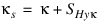
Formulas for the Longitudinal Force at Combined Slip
 | (80) |
with  the weighting function of the longitudinal force for pure slip.
the weighting function of the longitudinal force for pure slip.We write:
 | (81) |
 | (82) |
with coefficients:
 | (83) |
 | (84) |
 | (85) |
 | (86) |
 | (87) |
The weighting function follows as:
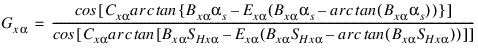 | (88) |
Longitudinal Force Coefficients at Combined Slip
Name: | Name used in tire property file: | Explanation: |
|---|---|---|
rBx1 | RBX1 | Slope factor for combined slip Fx reduction |
rBx2 | RBX2 | Variation of slope Fx reduction with kappa |
rCx1 | RCX1 | Shape factor for combined slip Fx reduction |
rEx1 | REX1 | Curvature factor of combined Fx |
rEx2 | REX2 | Curvature factor of combined Fx with load |
rHx1 | RHX1 | Shift factor for combined slip Fx reduction |
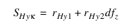
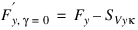
Formulas for Lateral Force at Combined Slip
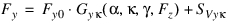 | (89) |
with Gyk the weighting function for the lateral force at pure slip and SVyk the ‘ -induced’ side force; therefore, the lateral force can be written as:
-induced’ side force; therefore, the lateral force can be written as: | (90) |
 | (91) |
with the coefficients:
 | (92) |
 | (93) |
 | (94) |
 | (95) |
 | (96) |
 | (97) |
 | (98) |
The weighting function appears is defined as:
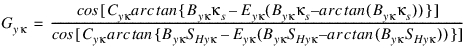 | (99) |
Lateral Force Coefficients at Combined Slip
Name: | Name used in tire property file: | Explanation: |
|---|---|---|
rBy1 | RBY1 | Slope factor for combined Fy reduction |
rBy2 | RBY2 | Variation of slope Fy reduction with alpha |
rBy3 | RBY3 | Shift term for alpha in slope Fy reduction |
rCy1 | RCY1 | Shape factor for combined Fy reduction |
rEy1 | REY1 | Curvature factor of combined Fy |
rEy2 | REY2 | Curvature factor of combined Fy with load |
rHy1 | RHY1 | Shift factor for combined Fy reduction |
rHy2 | RHY2 | Shift factor for combined Fy reduction with load |
rVy1 | RVY1 | Kappa induced side force Svyk/Muy*Fz at Fznom |
rVy2 | RVY2 | Variation of Svyk/Muy*Fz with load |
rVy3 | RVY3 | Variation of Svyk/Muy*Fz with inclination |
rVy4 | RVY4 | Variation of Svyk/Muy*Fz with alpha |
rVy5 | RVY5 | Variation of Svyk/Muy*Fz with kappa |
rVy6 | RVY6 | Variation of Svyk/Muy*Fz with atan (kappa) |
Formulas for Aligning Moment at Combined Slip
 | (100) |
with:
 | (101) |
 | (102) |
 | (103) |
 | (104) |
 | (105) |
with the arguments:
 | (106) |
 | (107) |
 | (108) |
Aligning Moment Coefficients at Combined Slip
Name: | Name used in tire property file: | Explanation: |
|---|---|---|
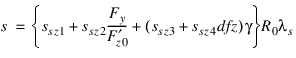
ssz1 | SSZ1 | Nominal value of s/R0 effect of Fx on Mz |
ssz2 | SSZ2 | Variation of distance s/R0 with Fy/Fznom |
ssz3 | SSZ3 | Variation of distance s/R0 with inclination |
ssz4 | SSZ4 | Variation of distance s/R0 with load and inclination |
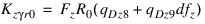
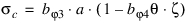
Formulas for Overturning Moment at Pure and Combined Slip
For the overturning moment, see also reference [5.], the formula reads both for pure and combined slip conditions:
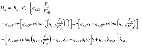 | (109) |
Overturning Moment Coefficients
Name: | Name used in tire property file: | Explanation: |
|---|---|---|
qsx1 | QSX1 | Vertical offset overturning couple |
qsx2 | QSX2 | Inclination induced overturning couple |
qsx3 | QSX3 | Fy induced overturning couple |
qsx4 | QSX4 | Fz induced overturning couple due to lateral tire deflection |
qsx5 | QSX5 | Fz induced overturning couple due to lateral tire deflection |
qsx6 | QSX6 | Fz induced overturning couple due to lateral tire deflection |
qsx7 | QSX7 | Fz induced overturning couple due to lateral tire deflection by inclination |
qsx8 | QSX8 | Fz induced overturning couple due to lateral tire deflection by lateral force |
qsx9 | QSX9 | Fz induced overturning couple due to lateral tire deflection by lateral force |
qsx10 | QSX10 | Inclination induced overturning couple, load dependency |
qsx11 | QSX11 | load dependency inclination induced overturning couple |
qpx1 | QPX1 | Variation of camber effect with pressure |
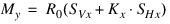
Formulas for Rolling Resistance Moment at Pure and Combined Slip
The rolling resistance moment is defined by:
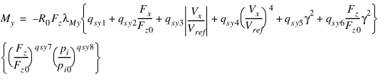 | (110) |
If qsy1 and qsy2 are both zero and FITTYP is equal to 5 (MF-Tyre 5.0), then the rolling resistance is calculated according to an old equation:
 | (111) |
Rolling Resistance Coefficients
Name: | Name used in tire property file: | Explanation: |
|---|---|---|
qsy1 | QSY1 | Rolling resistance moment coefficient |
qsy2 | QSY2 | Rolling resistance moment depending on Fx |
qsy3 | QSY3 | Rolling resistance moment depending on speed |
qsy4 | QSY4 | Rolling resistance moment depending on speed^4 |
qsy5 | QSY5 | Rolling resistance moment depending on camber |
qsy6 | QSY6 | Rolling resistance moment depending on camber and load |
qsy7 | QSY7 | Rolling resistance moment depending on load (exponential) |
qsy8 | QSY8 | Rolling resistance moment depending on inflation pressure |
Vref | LONGVL | Measurement speed |
Combined Slip with friction ellipse
In case the tire property file does not contain the coefficients for the 'standard' combined slip method (cosine 'weighing functions), the friction ellipse method is used, as described in this section.
Also the friction ellipse can be switched on by setting the keyword FE_METHOD in the [MODEL] section of the tire property file:
[MODEL]
FE_METHOD = 'YES'
Note that the method employed here is not part of one of the Magic Formula publications by Pacejka, but is an in-house development of MSC Software.
 | (112) |
 | (113) |
 | (114) |
 | (115) |
The following friction coefficients are defined:
 | (116) |
 | (117) |
 | (118) |
 | (119) |
The forces corrected for the combined slip conditions are:
 | (120) |
For aligning moment Mz, rolling resistance My and aligning moment Mz the formulae (76) until and including (85) are used with .
.
.Transient Behavior in PAC2002
The previous Magic Formula equations are valid for steady-state tire behavior. When driving, however, the tire requires some response time on changes of the inputs. In tire modeling terminology, the low-frequency behavior (up to 15 Hz) is called transient behavior. For modeling transient tire behavior PAC2002 provides two methods:
■Linear transient model (validity up to 8 Hz)
■Non linear transient model (validity up to 15 Hz)
In transient mode the tire model is able to deal with zero speed (stand-still). The more advanced non-linear transient mode shows better stand-still and tire spinning up performance. In combination with turn-slip and parking modeling, PAC2002 in non-linear transient mode is able to account for the so-called parking torque: the torque around the vertical axis due to the friction in between tire and road at stand-still when steering.
In the linear transient model, the longitudinal and lateral tire stiffness at stand-still depend on the rolling tire slip stiffness properties, while in the non-linear model the stand-still stiffness values depend on the carcass and slip stiffness properties, which is more realistic.
Linear transient model
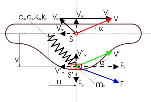
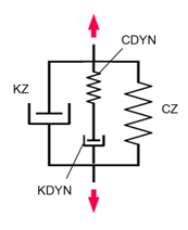
In the linear transient model the tire contact point S' is suspended to the wheel-rim plane with a longitudinal and lateral spring, with respectively stiffness's CFx and CFy, see reference [1]. In the figure below a top view of the tire with the single contact point S' and the longitudinal (u) and lateral (v) carcass deflections is shown.
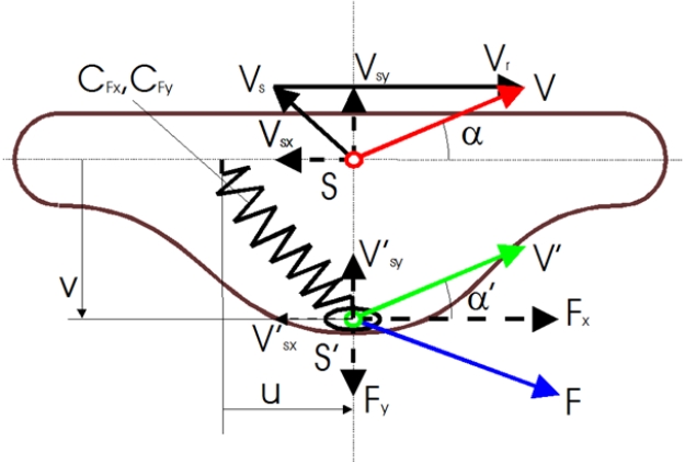
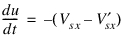
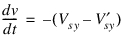
The contact point may move with respect to the wheel-rim plane and road. Movements relative to the road will result in tire-road interaction forces. Differences in slip velocities at point S and point S' will result in the tire carcass to deflect. The change of the longitudinal deflection u can be defined as:
 | (121) |
and the lateral deflection v as:
 | (122) |
For small values of slip the side force Fy can be calculated using the cornering stiffness CFα as follows:
 | (123) |
While the lateral force on the carcass reads:
 | (124) |
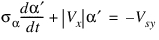
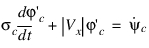
When introducing the lateral relaxation length σα as:
 | (125) |
the differential equation for the lateral deflection can be written as follows:
 | (126) |
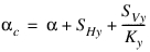
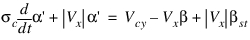
For linear small slip we can define the practical slip quantity α' as:
 | (127) |
With α' the equation for the lateral deflection becomes:
 | (128) |
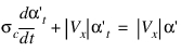
Similar the differential equation for longitudinal direction with the longitudinal relaxation length σκ can be derived:
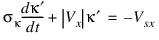 | (129) |
with the practical slip quantity κ'
 | (130) |
Both the longitudinal and lateral relaxation lengths are defined as of the vertical load:
 | (131) |
 | (132) |
Using these practical slip quantities, κ'and α', the Magic Formula equations can be used to calculate the transient tire-road interaction forces and moments:
 | (133) |
 | (134) |
 | (135) |
 | (136) |
 | (137) |
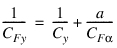
With this linear transient model the effective lateral compliance of the tire at stand-still is
 | (138) |
Similarly following applies for the longitudinal compliance:
 | (139) |
Coefficients of Linear Transient Model
Name: | Name used in tire property file: | Explanation: |
|---|---|---|
pTx1 | PTX1 | Longitudinal relaxation length at Fznom |
pTx2 | PTX2 | Variation of longitudinal relaxation length with load |
pTx3 | PTX3 | Variation of longitudinal relaxation length with exponent of load |
pTy1 | PTY1 | Peak value of relaxation length for lateral direction |
pTy2 | PTY2 | Shape factor for lateral relaxation length |
Non linear transient model
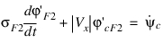
The contact mass model is based on the separation of the contact patch slip properties and the tire carcass compliance (see reference [1]). Instead of using relaxation lengths to describe compliance effects, the carcass springs are explicitly incorporated in the model. The contact patch is given some inertia to ensure computational causality. This modeling approach automatically accounts for the lagged response to slip and load changes that diminish at higher levels of slip. The contact patch itself uses relaxation lengths to handle simulations at low speed.
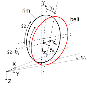
The contact patch can deflect in longitudinal, lateral, and yaw directions with respect to the lower part of the wheel rim. A mass is attached to the contact patch to enable straightforward computations. Note that the yaw deflection of the contact mass yaw β is not shown in the upper figure.
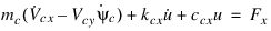
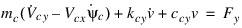
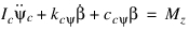
The differential equations that govern the dynamics of the contact patch body are:
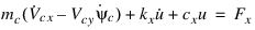 | (140) |
 | (141) |
 | (142) |
The contact patch body with mass mc and inertia Jc is connected to the wheel through springs cx, cy, and cψ and dampers kx, ky, and kψ in longitudinal, lateral, and yaw direction, respectively.
The additional equations for the longitudinal u, lateral v, and yaw β deflections are:
 | (143) |
 | (144) |
 | (145) |
in which Vcx, Vcy and  are the sliding velocity of the contact body in longitudinal, lateral, and yaw directions, respectively. Vsx, Vsy, and
  are the corresponding velocities of the lower part of the wheel.
are the sliding velocity of the contact body in longitudinal, lateral, and yaw directions, respectively. Vsx, Vsy, and are the corresponding velocities of the lower part of the wheel.The transient slip equations for side slip, turn-slip, and camber are:
 | (146) |
 | (147) |
 | (148) |
 | (149) |
 | (150) |
 | (151) |
 | (152) |
where the calculated deflection angle has been used:
 | (153) |
The tire total spin velocity is:
 | (154) |
With the transient slip equations, the composite transient turn-slip quantities are calculated:
 | (155) |
 | (156) |
The tire forces are calculated with  and the tire moments with
  .
.
and the tire moments with .The relaxation lengths are reduced with slip:
 | (157) |
 | (158) |
In which t0 is the pneumatic trail at zero slip angle.
 | (159) |
 | (160) |
 | (161) |
Here a is half the contact length according to:
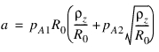 | (162) |
The composite tire parameter reads:
 | (163) |
and the equivalent slip  is calculated with the tire width b:
is calculated with the tire width b: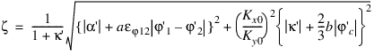 | (164) |
With the contact relaxation length σc equal to half the contact length (a), this advanced non-linear model will yield an effective lateral compliance CFy of the tire at stand-still equal to:
 | (165) |
The effective tire relaxation length for lateral slip (at zero lateral slip) results in:
 | (166) |
Similarly following applies for longitudinal direction (at zero longitudinal slip):
 | (167) |
One advantage of the non-linear transient above the linear transient model is the dependency of relaxation to the amount of slip: if the slip increases, the relaxation will decrease, see the plot below:
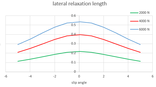
In order to have a better agreement with measurement data the longitudinal and lateral stiffness can be defined to be a function of load and slip:
 | (168) |
 | (169) |
 | (170) |
Coefficients of Non Linear Transient Model
Name: | Name used in tire property file: | Explanation: |
|---|---|---|
mc | MC | Contact body mass |
Ic | IC | Contact body moment of inertia |
kx | KX | Longitudinal damping |
ky | KY | Lateral damping |
kψ | KP | Yaw damping |
cx | CX | Longitudinal stiffness |
cy | CY | Lateral stiffness |
cψ | CP | Yaw stiffness |
cxz | CXZ1 | Longitudinal stiffness linear dependency on load |
cxz2 | CXZ2 | Longitudinal stiffness quadratic dependency on load |
cxx1 | CXX1 | Longitudinal stiffness dependency on long. slip |
cyz1 | CYZ1 | Lateral stiffness linear dependency on load |
cyz2 | CYZ2 | Lateral stiffness quadratic dependency on load |
cyy1 | CYY1 | Lateral stiffness dependency on lat. slip |
pA1 | PA1 | Half contact length with vertical tire deflection |
pA2 | PA2 | Half contact length with square root of vertical tire deflection |
 | EP | Composite turn-slip (moment) |
 | EP12 | Composite turn-slip (moment) increment |
bF2 | BF2 | Second relaxation length factor |
bϕ1 | BP1 | First moment relaxation length factor |
bϕ2 | BP2 | Second moment relaxation length factor |
bϕ3 | BP3 | Third moment relaxation factor |
bϕ4 | BP4 | Fourth moment relaxation factor |
The remaining contact mass model parameters are estimated automatically based on longitudinal and lateral stiffness specified in the tire property file.
PAC2002 with Belt Dynamics
The 'basic' PAC2002 tire model with the linear transient model (USE_MODE 11 - 14) is valid up to approximately 8 Hz. By switching to the (non-linear) advanced transient mode (USE_MODE 21 - 25) the validity of the tire model can be increased to 15 Hz.
However, for having accurate tire response for frequencies higher than the 15 Hz, for example in case of vehicle ride analysis or vehicle behavior with chassis control systems, the dynamics of the tire belt starts to play a role. PAC2002 also offers a feature to describe the lowest eigen modes of the belt by assuming the belt as a rigid ring (rigid body part). The modeling approach has been published by Pacejka and others [1,6-8] and comes down to the following:
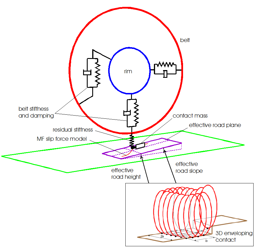
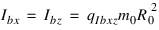
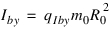
The wheel - tire assembly exists of a rim part and a belt part. In between the rim and the belt, a six degree of freedom bushing with stiffness and damping will allow the belt to move with respect to the rim. In between the belt and the road, the residual stiffness will contribute to a correct vertical overall stiffness of the tire.
The input from the road to the tire in terms of the effective road height, road angle and road camber is supplied by the 3D Enveloping Contact. The road-belt friction interaction forces are calculated with the Non linear transient model (contact mass approach) in combination the Magic Formula equations for the tire's Force & Moment response.
Running the PAC2002 with the belt dynamics option will leverage the validity range of the tire model towards appr. 70 - 80 Hz.
Rim - Belt bushing
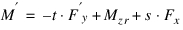
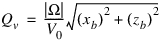
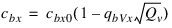
The interaction forces and torques in between the rim part and the wheel part are defined by a bushing with stiffness and damping forces in all 6 directions, x, y, z, γ, θ and ψ:
 | (171) |
 | (172) |
 | (173) |
 | (174) |
 | (175) |
 | (176) |
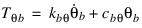
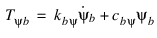
For introducing an effect of the belt deflection and the wheel rotational speed on the sidewall stiffness the variable quantity Qv is defined:
 | (177) |
with
 | (178) |
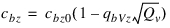 | (179) |
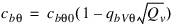 | (180) |
The non-dimensional belt stiffness rates qcbx, qcby, qcbz, qcbγ, qcbθ and qcbψ, to be supplied in the tire property file, are given by:
 | (181) |
 | (182) |
Because of the wheel symmetry following is valid:
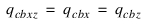 and
and 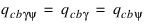
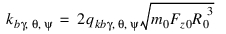
Similar, the non-dimensional qkbx, qkby, qkbz, qkbγ, qkbθ and qkbψ, damping rates have following relation to the parameters in the bushing force equations:
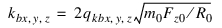 | (183) |
 | (184) |
in which
■R0 is the unloaded rolling radius of the tire.
■m0 is the mass of the tire.
■Fz0 is the nominal tire load.
Note that the in-plane damping parameters are equal due to the wheel symmetry:
 and
and 
The mass of the belt is defined with parameter qmb:
 | (185) |
and for the inertia of the belt qIbxz and qIby is used:
 | (186) |
 | (187) |
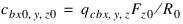
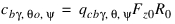
Normal load calculation
Knowing the deflection of the belt the vertical residual stiffness is calculated so that the tire overall normal load is still equal to the load defined in Equation (8) of the section "Contact Methods and Normal Load Calculation":
 | (188) |
Belt - Contact Mass
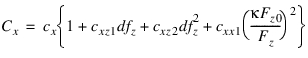
As mentioned, in the contact between the belt and the road, the non-linear transient model (see also section Non linear transient model, Equation (140) up to and including Equation (142)) is used, but with following parameters for the stiffness and damping:
 | (189) |
 | (190) |
 | (191) |
with
 | (192) |
 | (193) |
 | (194) |
 | (195) |
 | (196) |
 | (197) |
The contact mass is defined with parameter qmc:
 | (198) |
And the contact mass inertia is defined with qIc:
 | (199) |
Belt parameters
Name: | Name used in tire property file: | Explanation: |
|---|---|---|
m0 | TYRE_MASS | Mass of the tire |
qmb | QMB | Mass parameter of the tire belt |
qmc | QMC | Mass parameter of the tire contact mass |
qIbxz | QIBXZ | Ixx/Izz inertia parameter of the tire belt |
qIby | QIBY | Iyy inertia parameter of the tire belt |
qIc | QIC | Inertia parameter of the contact mass |
qcbxz | QCBXZ | Radial belt - wheel stiffness factor |
qcby | QCBY | Axial belt - wheel stiffness factor |
qcbγψ | QCBGM | Rotational belt - wheel stiffness factor |
qcbθ | QCBTH | Torsional belt - wheel stiffness factor |
qkbxz | QKBXZ | Radial belt - wheel damping factor |
qkby | QKBY | Axial belt - wheel damping factor |
qkbγψ | QKBGM | Rotational belt - wheel damping factor |
qkbθ | QKBTH | Torsional belt - wheel damping factor |
qbVxz | QBVXZ | Speed effect on radial belt - wheel stiffness |
qbVθ | QBVTH | Speed effect on torsional belt - wheel stiffness |
qccx | QCCX | Longitudinal stiffness factor belt - contact mass |
qccy | QCCY | Lateral stiffness factor belt - contact mass |
qccψ | QCCFI | Yaw stiffness factor belt - contact mass |
qkcx | QKCX | Longitudinal damping factor belt - contact mass |
qkcy | QKCY | Lateral damping factor belt - contact mass |
qkcψ | QKCFI | Yaw damping factor belt - contact mass |
PAC2002 Belt Parameters
The required parameters for running pac2002 with the belt dynamics option are:
■The Magic Formula parameters (steady state tire behavior). In the tire property file these are the sections LONGITUDINAL_COEFFICIENTS, OVERTURNING_COEFFICIENTS, LATERAL_COEFFICIENTS, ROLLING_COEFFICIENTS and ALIGNING_COEFFICIENTS.
■The parameters related to turn slip modeling, section TURNSLIP_COEFFICIENTS.
■The parameters related to the 3D Enveloping contact, section CONTACT_COEFFICIENTS. If these are not supplied, default values will be taken.
■And as last the new BELT_PARAMETERS. These define the parameters for the belt-rim bushing, and the contact mass (part of the non-linear transient model).
The belt dynamics feature can be switched on by the keyword BELT_DYNAMICS in the [MODEL] section of the tire property file, for example:
$----------------------------------------------------------------model
[MODEL]
PROPERTY_FILE_FORMAT = 'PAC2002'
USE_MODE = 14 $Tire use switch (IUSED)
LONGVL = 10.0 $Measurement speed at test bench (V0)
TYRESIDE = 'LEFT' $Mounted side at tire test bench
BELT_DYNAMICS = 'YES'
CONTACT_MODEL = '3D_ENVELOPING'
USE_MODE = 14 $Tire use switch (IUSED)
LONGVL = 10.0 $Measurement speed at test bench (V0)
TYRESIDE = 'LEFT' $Mounted side at tire test bench
BELT_DYNAMICS = 'YES'
CONTACT_MODEL = '3D_ENVELOPING'
$-----------------------------------------------------------dimensions
..
For Belt Dynamics an additional part is required for modelling the first belt eigenmodes with the rigid ring approach. For PAC2002 there are two options:
■The part for the belt is added to the Adams input deck. Using a bushing, the belt part is connected to the wheel part and the forces calculated by the tire model are applied to the belt. This option is activated if the keyword BELT_DYNAMCS is set to ‘YES’ or ‘EXTERNAL’.
■The part for the belt is evaluated within the tire model (no additional part in the Adams model is defined). The tire model calculates the forces to the wheel part. This option is activated if the keyword BELT_DYNAMCS is set to ‘INTERNAL’.
Having the belt part internal will require less states for Adams solver to integrate, this can have considerable advantages in case of real time applications. In the case of the internal belt part, all states for both the belt part and the tire differential equations can be solved by the tire local solver.
Though the USE_MODE is set to 14, internally the model will switch to USE_MODE 24.
When using a handling tire model in Adams, the tire-road interaction forces are applied on a (rotating) multi-body wheel part defined in the Adams Dataset. PAC2002 with belt dynamics needs one more multi-body part in the Adams Dataset: the belt part. Now the tire-road interaction forces will act on the belt part.
The Adams View and Adams Car preprocessors will recognize when PAC2002 is using the belt dynamics feature, and generate the multi-body belt part in the Adams Dataset.
In addition the total mass and inertia of the rim & wheel assembly as specified in the preprocessor will be distributed over the rim and belt part with the information from the PAC2002 tire property file.
An example tire property file with belt parameters is shown in the section Example of PAC2002 Tire Property Files.
Tire testing for belt parameters
The tire belt parameters should be identified out of tire test data performed under realistic tire operating conditions: for the belt parameters this means exciting the tire belt mode by rolling over road obstacles.
Most practical approach is using an external drum test bench, and roll the tire over a cleat at fixed axle height for various rotational speeds. The SAE standard J2730 [9] describes a proven concept for such a test program.
For identification of the PAC2002 belt parameters, the Adams Car Tire Test Rig can be used to reproduce the forces measured at cleat tests.
Parking Torque
The non-linear transient model in combination with the turn-slip / parking modeling (USE_MODE = 25) is able to account for the so-called parking torque at stand-still.
When applying a sine steering excitation to a standing tire in the non-linear (advanced) transient mode, the parking torque is generated around the vertical axis, as shown below.
The maximum parking torque is mainly determined by parameter qCrϕ1, while the stiffness is due to the yaw stiffness cψ value.
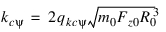
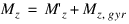
Gyroscopic Couple in PAC2002
When having fast rotations about the vertical axis in the wheel plane, the inertia of the tire belt may lead to gyroscopic effects. When using PAC2002 without the belt dynamics (USEMODE 10 - 25), there is still a simple approach to account for the gyroscopic effect. To cope with this additional moment, the following contribution is added to the total aligning moment:
 | (200) |
with the parameter (in addition to the basic tire parameter mbelt):
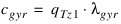 | (201) |
and:
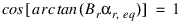 | (202) |
The total aligning moment now becomes:
 | (203) |
Coefficients of the Gyrocopic Couple
Name: | Name used in tire property file: | Explanation: |
|---|---|---|
qTz1 | QTZ1 | Gyroscopic moment constant |
Mbelt | MBELT | Belt mass of the wheel |
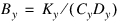
Non-rolling vertical tire stiffness and damping properties
In general the vertical stiffness and damping rates for a non-rolling tire differ from the stiffness and damping when rolling. In addition the non-rolling stiffness may depend on frequency. In the PAC2002 tire model a Maxwell element can be added to improve the non-rolling tire properties, for example for vehicle four poster simulations.
For using the Maxwell element the [VERTICAL] section of the tire property file should contain the keywords: USE_DYNAMIC_STIFFNESS, DYNAMIC_STIFFNESS and DYNAMIC_DAMPING, see the example snippet of a tire property file.
With USE_DYNAMIC_STIFFNESS = 'YES', the Maxwell element is switched on, with a ‘NO’ switched off.
Snippet of the [VERTICAL] section of a tire property file using the Maxwell element:
[VERTICAL]
VERTICAL_STIFFNESS = 2.1e+005
VERTICAL_DAMPING = 50
BREFF = 8.4
DREFF = 0.27
FREFF = 0.07
FNOMIN = 4850
USE_DYNAMIC_STIFFNESS = YES
DYNAMIC_STIFFNESS = 1.9E+003
DYNAMIC_DAMPING = 221
Left and Right Side Tires
In general, a tire produces a lateral force and aligning moment at zero slip angle due to the tire construction, known as conicity and plysteer. In addition, the tire characteristics cannot be symmetric for positive and negative slip angles.
A tire property file with the parameters for the model results from testing with a tire that is mounted in a tire test bench comparable either to the left or the right side of a vehicle. If these coefficients are used for both the left and the right side of the vehicle model, the vehicle does not drive straight at zero steering wheel angle.
The latest versions of tire property files contain a keyword TYRESIDE in the [MODEL] section that indicates for which side of the vehicle the tire parameters in that file are valid (TYRESIDE = 'LEFT' or TYRESIDE = 'RIGHT').
If this keyword is available, Adams Car corrects for the conicity and plysteer and asymmetry when using a tire property file on the opposite side of the vehicle. In fact, the tire characteristics are mirrored with respect to slip angle zero. In Adams View, this option can only be used when the tire is generated by the graphical user interface: select Build -> Forces -> Special Force: Tire.
Next to the LEFT and RIGHT side option of TYRESIDE, you can also set SYMMETRIC: then the tire characteristics are modified during initialization to show symmetric performance for left and right side corners and zero conicity and plysteer (no offsets).Also, when you set the tire property file to SYMMETRIC, the tire characteristics are changed to symmetric behavior.
Create Wheel and Tire Dialog Box in Adams View
Next to defining the mirroring via the GUI dialog window, also the USE_MODE parameter can be used: when the USE_MODE is negative, the tire characteristics will be mirrored as well.
When mirroring is done, following parameters will change sign:
RHX1, QSX1, PEY3, PHY1, PHY2, PVY1, PVY2, RBY3, RVY1, RVY2, QBZ4, QDZ3, QDZ6, QDZ7, QEZ4, QHZ1, QHZ2, SSZ1.
USE_MODES of PAC2002: from Simple to Complex
The parameter USE_MODE in the tire property file allows you to switch the output of the PAC2002 tire model from very simple (that is, steady-state cornering) to complex (transient combined cornering and braking).
The options for the USE_MODE and the output of the model have been listed in the table below.
USE_MODE Values of PAC2002 and Related Tire Model Output
USE_MODE: | State: | Slip conditions: | PAC2002 output (forces and moments): |
|---|---|---|---|
0 | Steady state | Acts as a vertical spring & damper | 0, 0, Fz, 0, 0, 0 |
1 | Steady state | Pure longitudinal slip | Fx, 0, Fz, 0, My, 0 |
2 | Steady state | Pure lateral (cornering) slip | 0, Fy, Fz, Mx, 0, Mz |
3 | Steady state | Longitudinal and lateral (not combined) | Fx, Fy, Fz, Mx, My, Mz |
4 | Steady state | Combined slip | Fx, Fy, Fz, Mx, My, Mz |
11 | Transient | Pure longitudinal slip | Fx, 0, Fz, 0, My, 0 |
12 | Transient | Pure lateral (cornering) slip | 0, Fy, Fz, Mx, 0, Mz |
13 | Transient | Longitudinal and lateral (not combined) | Fx, Fy, Fz, Mx, My, Mz |
14 | Transient | Combined slip | Fx, Fy, Fz, Mx, My, Mz |
21 | Advanced transient | Pure longitudinal slip | Fx, 0, Fz, My, 0 |
22 | Advanced transient | Pure lateral (cornering slip) | 0, Fy, Fz, Mx, 0, Mz |
23 | Advanced transient | Longitudinal and lateral (not combined) | Fx, Fy, Fz, Mx, My, Mz |
24 | Advanced transient | Combined slip | Fx, Fy, Fz, Mx, My, Mz |
25 | Advanced transient | Combined slip and turn-slip/parking | Fx, Fy, Fz, Mx, My, Mz |
In addition to the use mode, the BELT_DYNAMICS switch can be used for using the Belt Dynamics option. In that case the tire model will switch to USE_MODE 24 or 25 internally.
The local Tire Solver for increasing simulation speed
By default the differential states of the Adams Tire models are calculated by the General State Equation (GSE) as part of the Standard Tire Interface (STI). PAC2002 offers the option to calculate the state internally instead of passing this calculation to the Adams solver via the GSE. In particular when the number of states is large (advanced transient or belt dynamics), this will reduce the work load for the Adams Solver and will in many cases reduce the required CPU of the solver and thus increase simulation speed.
The use of this 'tire solver' is meant for simulations with rather small maximum time step: 0.005 s.
The use of the 'tire solver' can switched on by setting the LOCAL_SOLVER key word in the [MODEL] section of the tire property file:
$--------------------------------------------------------------model
[MODEL]
LOCAL_SOLVER = 'YES' $tire model is using a local calculation for the tire model states
If the local tire solver is activated in combination with zero tire states in the GSE (ac_tire UDE -> n_tire_states), the GSE will be de-activated in dynamics. For this purpose, environment variable MSC_ADAMS_INACTIVE_DYNAMICS, value="GSE, id_gse" is introduced in the Adams dataset.
High Performance switch in Adams Car
In the Adams Car tire subsystem file, the keyword 'HIGH_PERFORMANCE' can be set for the tire model. The default value for the keyword (when not present) is 'NO'. When the HIGH_PERFORMANCE is set to 'YES', the PAC2002 is set to a high performance mode which should reduce the required cpu of the simulation.
When HIGH_PERFORMANCE = 'YES', the keywords with extension _HP are taken instead of the base keyword, these are:
[MODEL]
LOCAL_SOLVER_HP = 'YES'
[CONTACT_COEFFICIENTS]
N_WIDTH_HP = 2
N_LENGTH_HP = 2
ROAD_SPACING_HP = 0.002 (mm)
Thus the LOCAL_SOLVER_HP setting will replace the LOCAL_SOLVER setting and so on. When the _HP settings are not defined, the upper mentions values are used by default.
One must take care to ensure that the proper balance between performance and accuracy is achieved when employing this new high performance mode.
Note that the LOCAL_SOLVER will be accurate for solver steps equal or smaller than 0.005 sec.
Examples:
1. The property file lists:
[MODEL]
LOCAL_SOLVER = 'YES'
[CONTACT_COEFFICIENTS]
ROAD_SPACING_HP = 0.002 (mm)
In this case the LOCAL_SOLVER will be used with high performance 'YES' and 'NO', the ROAD_SPACING will be set to 0.002 during high performance 'YES' only
2. The property file lists:
[MODEL]
LOCAL_SOLVER_HP = 'NO'
LOCAL_SOLVER_HP = 'YES'
In this case the LOCAL_SOLVER will be used with high performance 'YES' only.
PAC2002 support for DOE
PAC2002 offers the user to define a set of DOE parameters in the PAC2002 property file. Adams Car supports this functionality by creating an array for each tire containing these parameters and which are then referenced by Adams View Design Variables. These Design Variables can be used in for example, Adams Insight to changePAC2002 properties in design of experiments studies.
An example tire property file (acar/shared_car_database.cdb/tires.tbl/pac2002_235_60R16_doe.tir) is included in the Adams Car tire database. The section [DOE_PARAM_DEF] in the PAC2002 property file contains the names of the parameters which are chosen as DOE parameters, as shown below:
…
$------------------------------------------------------doe_param_def
[DOE_PARAM_DEF]
P1 = 'LKY'
P2 = 'PDY1'
P3 = 'RCY1'
$----------------------------------------------------------doe_param
[DOE_PARAM]
P1 = 1.0
P2 = 0.95
P3 = 1.04
…
When creating a tire in Adams Car, Creating a tire in Adams Car, the ac_tire UDE creates Adams View Design Variables based on the [DOE_PARAMETERS] section in the tire property file. For each tire, an array is created which references the Design Variables. The actual values of the DOE parameters defined in the [DOE_PARAM] are passed via this array (referenced by the 17th element of the tire input array) to the PAC2002 model.
Example doe array:
Object Name | : .MDI_Demo_Vehicle.TR_Front_Tires.til_wheel.doe_array |
Object Type | : Numbers ADAMS_Array |
Parent Type | : ac_tire |
Adams ID | : 902 |
Numbers | : 1.0 (.MDI_Demo_Vehicle.TR_Front_Tires.til_wheel.doe_p01) |
The design variables (for example, .MDI_Demo_Vehicle.TR_Front_Tires.til_wheel.doe_p01) can be used in for example, Adams Insight to perform studies varying PAC2002 properties.
Quality Checks for the Tire Model Parameters
Because PAC2002 uses an empirical approach to describe tire - road interaction forces, incorrect parameters can easily result in non-realistic tire behavior. Below is a list of the most important items to ensure the quality of the parameters in a tire property file:
Note: | Do not change Fz0 (FNOMIN) and R0 (UNLOADED_RADIUS) in your tire property file. It will change the complete tire characteristics because these two parameters are used to make all parameters without dimension. |
Rolling Resistance
For a realistic rolling resistance, the parameter qsy1 must be positive. For car tires, it can be in the order of 0.006 - 0.01 (0.6% - 1.0%); for heavy commercial truck tires, it can be around 0.006 (0.6%).
Tire property files with the keyword FITTYP=5 determine the rolling resistance in a different way (see equation (111)). To avoid the ‘old’ rolling resistance calculation, remove the keyword FITTYP and add a section like the following:
$---------------------------------------------------rolling resistance[ROLLING_COEFFICIENTS]
QSY1 = 0.01
QSY2 = 0
QSY3 = 0
QSY4 = 0
Camber (Inclination) Effects
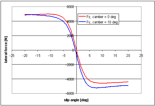
Camber stiffness has not been explicitly defined in PAC2002; however, for car tires, positive inclination should result in a negative lateral force at zero slip angle. If positive inclination results in an increase of the lateral force, the coefficient may not be valid for the ISO but for the SAE coordinate system. Note that PAC2002 only uses coefficients for the TYDEX W-axis (ISO) system.
Effect of Positive Camber on the Lateral Force in TYDEX W-axis (ISO) System
The table below lists further checks on the PAC2002 parameters.
Checklist for PAC2002 Parameters and Properties
Parameter/property: | Requirement: | Explanation: |
|---|---|---|
LONGVL | 1 m/s | Reference velocity at which parameters are measured |
VXLOW | Approximately 1 m/s | Threshold for scaling down forces and moments |
Dx | > 0 | Peak friction (see equation (23)) |
pDx1/pDx2 | < 0 | Peak friction Fx must decrease with increasing load |
Kx | > 0 | Long slip stiffness (see equation (26)) |
Dy | > 0 | Peak friction (see equation (35)) |
pDy1/pDy2 | < 0 | Peak friction Fx must decrease with increasing load |
Ky | < 0 | Cornering stiffness (see equation (38)) |
qsy1 | > 0 | Rolling resistance, in the range of 0.005 - 0.015 |
Validity Range of the Tire Model Input
In the tire property file, a range of the input variables has been given in which the tire properties are supposed to be valid. These validity range parameters are (the listed values can be different):
$--------------------------------------------------long_slip_range
[LONG_SLIP_RANGE]
KPUMIN = -1.5 $Minimum valid wheel slip
KPUMAX = 1.5 $Maximum valid wheel slip
$-------------------------------------------------slip_angle_range
[SLIP_ANGLE_RANGE]
ALPMIN = -1.5708 $Minimum valid slip angle
ALPMAX = 1.5708 $Maximum valid slip angle
$--------------------------------------------inclination_slip_range
[INCLINATION_ANGLE_RANGE]
CAMMIN = -0.26181 $Minimum valid camber angle
CAMMAX = 0.26181 $Maximum valid camber angle
$----------------------------------------------vertical_force_range
[VERTICAL_FORCE_RANGE]
FZMIN = 225 $Minimum allowed wheel load
FZMAX = 10125 $Maximum allowed wheel load
If one of the input parameters exceeds a minimum or maximum validity value, the calculation in the tire model is performed with the minimum or maximum value of this range to avoid non-realistic tire behavior. In that case, a message appears warning you that one of the inputs exceeds a validity value.
Standard Tire Interface (STI) for PAC2002
Because all Adams products use the Standard Tire Interface (STI) for linking the tire models to Adams Solver, below is a brief background of the STI history (see also reference [4]).
At the First International Colloquium on Tire Models for Vehicle Dynamics Analysis on October 21-22, 1991, the International Tire Workshop working group was established (TYDEX).
The working group concentrated on tire measurements and tire models used for vehicle simulation purposes. For most vehicle dynamics studies, people used to develop their own tire models. Because all car manufacturers and their tire suppliers have the same goal (that is, development of tires to improve dynamic safety of the vehicle) it aimed for standardization in tire behavior description.
In TYDEX, two expert groups, consisting of participants of vehicle industry (passenger cars and trucks), tire manufacturers, other suppliers and research laboratories, had been defined with following goals:
■The first expert group's (Tire Measurements - Tire Modeling) main goal was to specify an interface between tire measurements and tire models. The result was the TYDEX-Format [2] to describe tire measurement data.
■The second expert group's (Tire Modeling - Vehicle Modeling) main goal was to specify an interface between tire models and simulation tools, which resulted in the Standard Tire Interface (STI) [3]. The use of this interface should ensure that a wide range of simulation software can be linked to a wide range of tire modeling software.
Definitions
General
General Definitions
Term: | Definition: |
|---|---|
Road tangent plane | Plane with the normal unit vector (tangent to the road) in the tire-road contact point C. |
C-axis system | Coordinate system mounted on the wheel carrier at the wheel center according to TYDEX, ISO orientation. |
Wheel plane | The plane in the wheel center that is formed by the wheel when considered a rigid disc with zero width. |
Contact point C | Contact point between tire and road, defined as the intersection of the wheel plane and the projection of the wheel axis onto the road plane. |
W-axis system | Coordinate system at the tire contact point C, according to TYDEX, ISO orientation. |
Tire Kinematics
Tire Kinematics Definitions
Parameter: | Definition: | Units: |
|---|---|---|
R0 | Unloaded tire radius | [m] |
R | Loaded tire radius | [m] |
Re | Effective tire radius | [m] |
 | Radial tire deflection | [m] |
 | Dimensionless radial tire deflection | [-] |
 | Radial tire deflection at nominal load | [m] |
mbelt | Tire belt mass | [kg] |
 | Rotational velocity of the wheel | [radian-1] |
Slip Quantities
Slip Quantities Definitions
Parameter: | Definition: | Units: |
|---|---|---|
V | Vehicle speed | [ms-1] |
Vsx | Slip speed in x direction | [ms-1] |
Vsy | Slip speed in y direction | [ms-1] |
Vs | Resulting slip speed | [ms-1] |
Vx | Rolling speed in x direction | [ms-1] |
Vy | Lateral speed of tire contact center | [ms-1] |
Vr | Linear speed of rolling | [ms-1] |
 | Longitudinal slip | [-] |
 | Slip angle | [radian] |
 | Inclination angle | [radian] |
Forces and Moments
Force and Moment Definitions
Abbreviation: | Definition: | Units: |
|---|---|---|
Fz | Vertical wheel load | [N] |
Fz0 | Nominal load | [N] |
dfz | Dimensionless vertical load | [-] |
Fx | Longitudinal force | [N] |
Fy | Lateral force | [N] |
Mx | Overturning moment | [Nm] |
My | Braking/driving moment | [Nm] |
Mz | Aligning moment | [Nm] |
References
1. H.B. Pacejka, Tyre and Vehicle Dynamics, 2002, Butterworth-Heinemann, ISBN 0 7506 5141 5.
2. H.-J. Unrau, J. Zamow, TYDEX-Format, Description and Reference Manual, Release 1.1, Initiated by the International Tire Working Group, July 1995.
3. A. Riedel, Standard Tire Interface, Release 1.2, Initiated by the Tire Workgroup, June 1995.
4. J.J.M. van Oosten, H.-J. Unrau, G. Riedel, E. Bakker, TYDEX Workshop: Standardisation of Data Exchange in Tyre Testing and Tyre Modelling, Proceedings of the 2nd International Colloquium on Tyre Models for Vehicle Dynamics Analysis, Vehicle System Dynamics, Volume 27, Swets & Zeitlinger, Amsterdam/Lisse, 1996.
5. L. Merkx, Overturning moment analysis using the Flat plank tyre tester, DCT 2004-78, Department of Mechanical Engineering, University of Technology Eindhoven.
6. A.J.C. Schmeitz, "A semi-empirical three-dimensional model of the pneumatic tyre rolling over arbitrary uneven road surfaces," Ph.D. thesis, Delft University of Technology, Delft, 2004.
7. Maurice, J.P., "Short Wavelength and Dynamic Tyre Behaviour under Later and Combined Slip Conditions", PhD Thesis, Delft University of Technology, Delft, 2000.
8. Zegelaar, P.W.A., "The Dynamic Response of Tyres to Brake Torque Variations and Road Unevenesses", PhD Thesis, Delft University of Technology, Delft, 1998.
9. "Dynamic Cleat Test with Perpendicular and Inclined Cleats", SAE Standard J2730.
Example of PAC2002 Tire Property Files
Example of a tire property file with linear transient (USE_MODE = 14):
[MDI_HEADER]
FILE_TYPE ='tir'
FILE_VERSION =3.0
FILE_FORMAT ='ASCII'
! : TIRE_VERSION : PAC2002
! : COMMENT : Tire 235/60R16
! : COMMENT : Manufacturer
! : COMMENT : Nom. section with (m) 0.235
! : COMMENT : Nom. aspect ratio (-) 60
! : COMMENT : Infl. pressure (Pa) 200000
! : COMMENT : Rim radius (m) 0.19
! : COMMENT : Measurement ID
! : COMMENT : Test speed (m/s) 16.6
! : COMMENT : Road surface
! : COMMENT : Road condition Dry
! : FILE_FORMAT : ASCII
! : Copyright (C) 2004-2011 MSC Software Corporation
!
! USE_MODE specifies the type of calculation performed:
! 0: Fz only, no Magic Formula evaluation
! 1: Fx,My only
! 2: Fy,Mx,Mz only
! 3: Fx,Fy,Mx,My,Mz uncombined force/moment calculation
! 4: Fx,Fy,Mx,My,Mz combined force/moment calculation
! +10: including relaxation behaviour
! 15: Fx,Fy,Mx,My,Mz combined force/moment calculation, relaxation behaviour, including turn-slip torque
! +20: including advanced transient (contact mass approach)
! 25: Fx,Fy,Mx,My,Mz combined force/moment calculation, advanced transient including turn-slip torque & parking torque
! *-1: mirroring of tyre characteristics
!
! example: USE_MODE = -12 implies:
! -calculation of Fy,Mx,Mz only
! -including relaxation effects
! -mirrored tyre characteristics
!
$----------------------------------------------------------------units
[UNITS]
LENGTH ='meter'
FORCE ='newton'
ANGLE ='radian'
MASS ='kg'
TIME ='second'
$----------------------------------------------------------------model
[MODEL]
PROPERTY_FILE_FORMAT ='PAC2002' $Tire property type
USE_MODE = 14 $Tyre use switch (IUSED)
VXLOW = 1 $Below this speed forces are scaled down
LONGVL = 16.6 $Measurement speed
FE_METHOD = 'NO' $For switching to Friction ellipse for combined slip
TYRESIDE = 'LEFT' $Mounted side of tyre at vehicle/test bench
$-----------------------------------------------------------dimensions
[DIMENSION]
UNLOADED_RADIUS = 0.344 $Free tyre radius
WIDTH = 0.235 $Nominal section width of the tyre
ASPECT_RATIO = 0.6 $Nominal aspect ratio
RIM_RADIUS = 0.19 $Nominal rim radius
RIM_WIDTH = 0.16 $Rim width
$-----------------------------------------------------------load_curve
$ For a non-linear tire vertical stiffness
$ Maximum of 100 points
[DEFLECTION_LOAD_CURVE]
{pen fz}
0.000 0.0
0.001 212.0
0.002 428.0
0.003 648.0
0.005 1100.0
0.010 2300.0
0.020 5000.0
0.030 8100.0
$-------------------------------------------------------------RIMPACT_CURVE
$ Maximum of 100 points
[BOTTOMING_CURVE]
{pen fz}
0.0 0.0
0.09 0.0
0.1 100000.0
0.2 200000.0
0.3 300000.0
0.4 400000.0
0.5 500000.0
0.6 600000.0
6.0 6000000.0
0.09 0.0
0.1 100000.0
0.2 200000.0
0.3 300000.0
0.4 400000.0
0.5 500000.0
0.6 600000.0
6.0 6000000.0
$------------------------------------------------------------parameter
[VERTICAL]
VERTICAL_STIFFNESS = 2.1e+005 $Tyre vertical stiffness
VERTICAL_DAMPING = 50 $Tyre vertical damping
BREFF = 8.4 $Low load stiffness e.r.r.
DREFF = 0.27 $Peak value of e.r.r.
FREFF = 0.07 $High load stiffness e.r.r.
FNOMIN = 4850 $Nominal wheel load
VERTICAL_DAMPING = 50 $Tyre vertical damping
BREFF = 8.4 $Low load stiffness e.r.r.
DREFF = 0.27 $Peak value of e.r.r.
FREFF = 0.07 $High load stiffness e.r.r.
FNOMIN = 4850 $Nominal wheel load
$------------------------------------------------------long_slip_range
[LONG_SLIP_RANGE]
KPUMIN = -1.5 $Minimum valid wheel slip
KPUMAX = 1.5 $Maximum valid wheel slip
KPUMAX = 1.5 $Maximum valid wheel slip
$-----------------------------------------------------slip_angle_range
[SLIP_ANGLE_RANGE]
ALPMIN = -1.5708 $Minimum valid slip angle
ALPMAX = 1.5708 $Maximum valid slip angle
$-----------------------------------------------inclination_slip_range
[INCLINATION_ANGLE_RANGE]
CAMMIN = -0.26181 $Minimum valid camber angle
CAMMAX = 0.26181 $Maximum valid camber angle
$-------------------------------------------------vertical_force_range
[VERTICAL_FORCE_RANGE]
FZMIN = 225 $Minimum allowed wheel load
FZMAX = 10125 $Maximum allowed wheel load
$--------------------------------------------------------------scaling
[SCALING_COEFFICIENTS]
LFZO = 1 $Scale factor of nominal (rated) load
LCX = 1 $Scale factor of Fx shape factor
LMUX = 1 $Scale factor of Fx peak friction coefficient
LEX = 1 $Scale factor of Fx curvature factor
LKX = 1 $Scale factor of Fx slip stiffness
LHX = 1 $Scale factor of Fx horizontal shift
LVX = 1 $Scale factor of Fx vertical shift
LGAX = 1 $Scale factor of camber for Fx
LCY = 1 $Scale factor of Fy shape factor
LMUY = 1 $Scale factor of Fy peak friction coefficient
LEY = 1 $Scale factor of Fy curvature factor
LKY = 1 $Scale factor of Fy cornering stiffness
LHY = 1 $Scale factor of Fy horizontal shift
LVY = 1 $Scale factor of Fy vertical shift
LGAY = 1 $Scale factor of camber for Fy
LTR = 1 $Scale factor of Peak of pneumatic trail
LRES = 1 $Scale factor for offset of residual torque
LGAZ = 1 $Scale factor of camber for Mz
LXAL = 1 $Scale factor of alpha influence on Fx
LYKA = 1 $Scale factor of alpha influence on Fx
LVYKA = 1 $Scale factor of kappa induced Fy
LS = 1 $Scale factor of Moment arm of Fx
LSGKP = 1 $Scale factor of Relaxation length of Fx
LSGAL = 1 $Scale factor of Relaxation length of Fy
LGYR = 1 $Scale factor of gyroscopic torque
LMX = 1 $Scale factor of overturning couple
LVMX = 1 $Scale factor of Mx vertical shift
LMY = 1 $Scale factor of rolling resistance torque
$---------------------------------------------------------longitudinal
[LONGITUDINAL_COEFFICIENTS]
PCX1 = 1.6411 $Shape factor Cfx for longitudinal force
PDX1 = 1.1739 $Longitudinal friction Mux at Fznom
PDX2 = -0.16395 $Variation of friction Mux with load
PDX3 = 0 $Variation of friction Mux with camber
PEX1 = 0.46403 $Longitudinal curvature Efx at Fznom
PEX2 = 0.25022 $Variation of curvature Efx with load
PEX3 = 0.067842 $Variation of curvature Efx with load squared
PEX4 = -3.7604e-005 $Factor in curvature Efx while driving
PKX1 = 22.303 $Longitudinal slip stiffness Kfx/Fz at Fznom
PKX2 = 0.48896 $Variation of slip stiffness Kfx/Fz with load
PKX3 = 0.21253 Exponent in slip stiffness Kfx/Fz with load
PHX1 = 0.0012297 $Horizontal shift Shx at Fznom
PHX2 = 0.0004318 $Variation of shift Shx with load
PVX1 = -8.8098e-006 $Vertical shift Svx/Fz at Fznom
PVX2 = 1.862e-005 $Variation of shift Svx/Fz with load
RBX1 = 13.276 $Slope factor for combined slip Fx reduction
RBX2 = -13.778 $Variation of slope Fx reduction with kappa
RCX1 = 1.2568 $Shape factor for combined slip Fx reduction
REX1 = 0.65225 $Curvature factor of combined Fx
REX2 = -0.24948 $Curvature factor of combined Fx with load
RHX1 = 0.0050722 $Shift factor for combined slip Fx reduction
PTX1 = 2.3657 $Relaxation length SigKap0/Fz at Fznom
PTX2 = 1.4112 $Variation of SigKap0/Fz with load
PTX3 = 0.56626 $Variation of SigKap0/Fz with exponent of load
$----------------------------------------------------------overturning
[OVERTURNING_COEFFICIENTS]
QSX1 = 0 $Vertical offset overturning moment
QSX2 = 0 $Camber induced overturning couple
QSX3 = 0 $Fy induced overturning couple
$--------------------------------------------------------------lateral
[LATERAL_COEFFICIENTS]
PCY1 = 1.3507 $Shape factor Cfy for lateral forces
PDY1 = 1.0489 $Lateral friction Muy
PDY2 = -0.18033 $Variation of friction Muy with load
PDY3 = -2.8821 $Variation of friction Muy with squared camber
PEY1 = -0.0074722 $Lateral curvature Efy at Fznom
PEY2 = -0.0063208 $Variation of curvature Efy with load
PEY3 = -9.9935 $Zero order camber dependency of curvature Efy
PEY4 = -760.14 $Variation of curvature Efy with camber
PKY1 = -21.92 $Maximum value of stiffness Kfy/Fznom
PKY2 = 2.0012 $Load at which Kfy reaches maximum value
PKY3 = -0.024778 $Variation of Kfy/Fznom with camber
PHY1 = 0.0026747 $Horizontal shift Shy at Fznom
PHY2 = 8.9094e-005 $Variation of shift Shy with load
PHY3 = 0.031415 $Variation of shift Shy with camber
PVY1 = 0.037318 $Vertical shift in Svy/Fz at Fznom
PVY2 = -0.010049 $Variation of shift Svy/Fz with load
PVY3 = -0.32931 $Variation of shift Svy/Fz with camber
PVY4 = -0.69553 $Variation of shift Svy/Fz with camber and load
RBY1 = 7.1433 $Slope factor for combined Fy reduction
RBY2 = 9.1916 $Variation of slope Fy reduction with alpha
RBY3 = -0.027856 $Shift term for alpha in slope Fy reduction
RCY1 = 1.0719 $Shape factor for combined Fy reduction
REY1 = -0.27572 $Curvature factor of combined Fy
REY2 = 0.32802 $Curvature factor of combined Fy with load
RHY1 = 5.7448e-006 $Shift factor for combined Fy reduction
RHY2 = -3.1368e-005 $Shift factor for combined Fy reduction with load
RVY1 = -0.027825 $Kappa induced side force Svyk/Muy*Fz at Fznom
RVY2 = 0.053604 $Variation of Svyk/Muy*Fz with load
RVY3 = -0.27568 $Variation of Svyk/Muy*Fz with camber
RVY4 = 12.12 $Variation of Svyk/Muy*Fz with alpha
RVY5 = 1.9 $Variation of Svyk/Muy*Fz with kappa
RVY6 = -10.704 $Variation of Svyk/Muy*Fz with atan(kappa)
PTY1 = 2.1439 $Peak value of relaxation length SigAlp0/R0
PTY2 = 1.9829 $Value of Fz/Fznom where SigAlp0 is extreme
$---------------------------------------------------rolling resistance
[ROLLING_COEFFICIENTS]
QSY1 = 0.01 $Rolling resistance torque coefficient
QSY2 = 0 $Rolling resistance torque depending on Fx
QSY3 = 0 $Rolling resistance torque depending on speed
QSY4 = 0 $Rolling resistance torque depending on speed ^4
$-------------------------------------------------------------aligning
[ALIGNING_COEFFICIENTS]
QBZ1 = 10.904 $Trail slope factor for trail Bpt at Fznom
QBZ2 = -1.8412 $Variation of slope Bpt with load
QBZ3 = -0.52041 $Variation of slope Bpt with load squared
QBZ4 = 0.039211 $Variation of slope Bpt with camber
QBZ5 = 0.41511 $Variation of slope Bpt with absolute camber
QBZ9 = 8.9846 $Slope factor Br of residual torque Mzr
QBZ10 = 0 $Slope factor Br of residual torque Mzr
QCZ1 = 1.2136 $Shape factor Cpt for pneumatic trail
QDZ1 = 0.093509 $Peak trail Dpt" = Dpt*(Fz/Fznom*R0)
QDZ2 = -0.0092183 $Variation of peak Dpt" with load
QDZ3 = -0.057061 $Variation of peak Dpt" with camber
QDZ4 = 0.73954 $Variation of peak Dpt" with camber squared
QDZ6 = -0.0067783 $Peak residual torque Dmr" = Dmr/(Fz*R0)
QDZ7 = 0.0052254 $Variation of peak factor Dmr" with load
QDZ8 = -0.18175 $Variation of peak factor Dmr" with camber
QDZ9 = 0.029952 $Variation of peak factor Dmr" with camber and load
QEZ1 = -1.5697 $Trail curvature Ept at Fznom
QEZ = 0.33394 $Variation of curvature Ept with load
QEZ3 = 0 $Variation of curvature Ept with load squared
QEZ4 = 0.26711 $Variation of curvature Ept with sign of Alpha-t
QEZ5 = -3.594 $Variation of Ept with camber and sign Alpha-t
QHZ1 = 0.0047326 $Trail horizontal shift Sht at Fznom
QHZ2 = 0.0026687 $Variation of shift Sht with load
QHZ3 = 0.11998 $Variation of shift Sht with camber
QHZ4 = 0.059083 $Variation of shift Sht with camber and load
SSZ1 = 0.033372 $Nominal value of s/R0: effect of Fx on Mz
SSZ2 = 0.0043624 $Variation of distance s/R0 with Fy/Fznom
SSZ3 = 0.56742 $Variation of distance s/R0 with camber
SSZ4 = -0.24116 $Variation of distance s/R0 with load and camber
QTZ1 = 0.2 $Gyration torque constant
MBELT = 5.4 $Belt mass of the wheel
$-----------------------------------------------turn-slip parameters
[TURNSLIP_COEFFICIENTS]
PECP1 = 0.7 $Camber stiffness reduction factor
PECP2 = 0.0 $Camber stiffness reduction factor with load
PDXP1 = 0.4 $Peak Fx reduction due to spin
PDXP2 = 0.0 $Peak Fx reduction due to spin with load
PDXP3 = 0.0 $Peak Fx reduction due to spin with longitudinal slip
PDYP1 = 0.4 $Peak Fy reduction due to spin
PDYP2 = 0.0 $Peak Fy reduction due to spin with load
PDYP3 = 0.0 $Peak Fy reduction due to spin with lateral slip
PDYP4 = 0.0 $Peak Fy reduction with square root of spin
PKYP1 = 1.0 $Cornering stiffness reduction due to spin
PHYP1 = 1.0 $Fy lateral shift shape factor
PHYP2 = 0.15 $Maximum Fy lateral shift
PHYP3 = 0.0 $Maximum Fy lateral shift with load
PHYP4 = -4.0 $Fy lateral shift curvature factor
QDTP1 = 10.0 $Pneumatic trail reduction factor
QBRP1 = 0.1 $Residual torque reduction factor with lateral slip
QCRP1 = 0.2 $Turning moment at constant turning with zero speed
QCRP2 = 0.1 $Turning moment at 90 deg lateral slip
QDRP1 = 1.0 $Maximum turning moment
QDRP2 = -1.5 $Location of maximum turning moment
$-----------------------------------------------contact patch parameters
[CONTACT_COEFFICIENTS]
PA1 = 0.4147 $Half contact length dependency on sqrt(Fz/Fz0)
PA2 = 1.9129 $Half contact length dependency on Fz
$-----------------------------------------------contact patch slip model
[DYNAMIC_COEFFICIENTS]
MC = 1.0 $Contact mass
IC = 0.05 $Contact moment of inertia
KX = 409.0 $Contact longitudinal damping
KY = 320.8 $Contact lateral damping
KP = 11.9 $Contact yaw damping
CX = 4.350e+005 $Contact longitudinal stiffness
CY = 1.665e+005 $Contact lateral stiffness
CP = 20319 $Contact yaw stiffness
EP = 1.0
EP12 = 4.0
BF2 = 0.5
BP1 = 0.5
BP2 = 0.67
$------------------------------------------------------loaded radius
[LOADED_RADIUS_COEFFICIENTS]
QV1 = 0.000071 $Tire radius growth coefficient
QV2 = 2.489 $Tire stiffness variation coefficient with speed
QFCX1 = 0.1 $Tire stiffness interaction with Fx
QFCY1 = 0.3 $Tire stiffness interaction with Fy
QFCG1 = 0.0 $Tire stiffness interaction with camber
QFZ1 = 0.0 $Linear stiffness coefficient, if zero, VERTICAL_STIFFNESS is taken
QFZ2 = 14.35 $Tire vertical stiffness coefficient (quadratic)
Example of a tire property file with belt dynamics:
[MDI_HEADER]
FILE_TYPE ='tir'
FILE_VERSION =3.0
FILE_FORMAT ='ASCII'
! : TIRE_VERSION : PAC2002
! : COMMENT : Tire 205/55 R16
! : COMMENT : Manufacturer -
! : COMMENT : Nom. section width (m) 0.205
! : COMMENT : Nom. aspect ratio (-) 55
! : COMMENT : Infl. pressure (Pa) 250000
! : COMMENT : Rim radius (m) 0.203
! : COMMENT : Measurement ID
! : COMMENT : Test speed (m/s) 30
! : COMMENT : Road surface
! : COMMENT : Road condition
! : FILE_FORMAT : ASCII
! : Copyright (C) 2004-2011 MSC Software Corporation
!
! USE_MODE specifies the type of calculation performed:
! 0: Fz only, no Magic Formula evaluation
! 1: Fx,My only
! 2: Fy,Mx,Mz only
! 3: Fx,Fy,Mx,My,Mz uncombined force/moment calculation
! 4: Fx,Fy,Mx,My,Mz combined force/moment calculation
! +10: including relaxation behaviour
! 15: Fx,Fy,Mx,My,Mz combined force/moment calculation, relaxation behaviour, including turn-slip torque
! +20: including advanced transient (contact mass approach)
! 25: Fx,Fy,Mx,My,Mz combined force/moment calculation, advanced transient including turn-slip torque & parking torque
! *-1: mirroring of tire characteristics
!
! when beltdynamics is switched on the usemode will be 24 or 25
!
! example: USE_MODE = -12 implies:
! -calculation of Fy,Mx,Mz only
! -including relaxation effects
! -mirrored tire characteristics
!
$----------------------------------------------------------------units
[UNITS]
LENGTH ='meter'
FORCE ='newton'
ANGLE ='radian'
MASS ='kg'
TIME ='second'
FORCE ='newton'
ANGLE ='radian'
MASS ='kg'
TIME ='second'
$----------------------------------------------------------------model
[MODEL]
PROPERTY_FILE_FORMAT = 'PAC2002'
USE_MODE = 14 $Tire use switch (IUSED)
LONGVL = 10.0 $Measurement speed at test bench (V0)
TYRESIDE = 'LEFT' $Mounted side at tire test bench LEFT/RIGHT/SYMMETRIC
BELT_DYNAMICS = 'YES'
CONTACT_MODEL = '3D_ENVELOPING'
USE_MODE = 14 $Tire use switch (IUSED)
LONGVL = 10.0 $Measurement speed at test bench (V0)
TYRESIDE = 'LEFT' $Mounted side at tire test bench LEFT/RIGHT/SYMMETRIC
BELT_DYNAMICS = 'YES'
CONTACT_MODEL = '3D_ENVELOPING'
$-----------------------------------------------------------dimensions
[DIMENSION]
UNLOADED_RADIUS = 0.3169 $Free tire radius
WIDTH = 0.205 $Nominal section width of the tire
ASPECT_RATIO = 0.55 $Nominal aspect ratio
RIM_RADIUS = 0.203 $Nominal rim radius
RIM_WIDTH = 0.165 $Rim width
$----------------------------------------------------------------shape
[SHAPE]
{radial width}
1.0 0.0
1.0 0.4
1.0 0.9
0.9 1.0
$------------------------------------------------------------parameter
[VERTICAL]
VERTICAL_STIFFNESS = 209200.0 $Tire vertical stiffness
VERTICAL_DAMPING = 500 $Tire vertical damping
BREFF = 4.90 $Low load stiffness e.r.r.
DREFF = 0.41 $Peak value of e.r.r.
FREFF = 0.09 $High load stiffness e.r.r.
FNOMIN = 4700 $Nominal wheel load
$------------------------------------------------------long_slip_range
[LONG_SLIP_RANGE]
KPUMIN = -1.5 $Minimum valid wheel slip
KPUMAX = 1.5 $Maximum valid wheel slip
$-----------------------------------------------------slip_angle_range
[SLIP_ANGLE_RANGE]
ALPMIN = -1.5708 $Minimum valid slip angle
ALPMAX = 1.5708 $Maximum valid slip angle
$-----------------------------------------------inclination_slip_range
[INCLINATION_ANGLE_RANGE]
CAMMIN = -0.26181 $Minimum valid camber angle
CAMMAX = 0.26181 $Maximum valid camber angle
$-------------------------------------------------vertical_force_range
[VERTICAL_FORCE_RANGE]
FZMIN = 140 $Minimum allowed wheel load
FZMAX = 10800 $Maximum allowed wheel load
$--------------------------------------------------------------scaling
[SCALING_COEFFICIENTS]
LFZO = 1 $Scale factor of nominal (rated) load
LCX = 1 $Scale factor of Fx shape factor
LMUX = 1 $Scale factor of Fx peak friction coefficient
LEX = 1 $Scale factor of Fx curvature factor
LKX = 1 $Scale factor of Fx slip stiffness
LHX = 1 $Scale factor of Fx horizontal shift
LVX = 1 $Scale factor of Fx vertical shift
LGAX = 1 $Scale factor of camber for Fx
LCY = 1 $Scale factor of Fy shape factor
LMUY = 1 $Scale factor of Fy peak friction coefficient
LEY = 1 $Scale factor of Fy curvature factor
LKY = 1 $Scale factor of Fy cornering stiffness
LHY = 1 $Scale factor of Fy horizontal shift
LVY = 1 $Scale factor of Fy vertical shift
LGAY = 1 $Scale factor of camber for Fy
LTR = 1 $Scale factor of Peak of pneumatic trail
LRES = 1 $Scale factor for offset of residual torque
LGAZ = 1 $Scale factor of camber for Mz
LXAL = 1 $Scale factor of alpha influence on Fx
LYKA = 1 $Scale factor of alpha influence on Fx
LVYKA = 1 $Scale factor of kappa induced Fy
LS = 1 $Scale factor of Moment arm of Fx
LSGKP = 1 $Scale factor of Relaxation length of Fx
LSGAL = 1 $Scale factor of Relaxation length of Fy
LGYR = 1 $Scale factor of gyroscopic torque
LMX = 1 $Scale factor of overturning couple
LVMX = 1 $Scale factor of Mx vertical shift
LMY = 1 $Scale factor of rolling resistance torque
$---------------------------------------------------------longitudinal
[LONGITUDINAL_COEFFICIENTS]
PCX1 = 1.3178 $Shape factor Cfx for longitudinal force
PDX1 = 1.0455 $Longitudinal friction Mux at Fznom
PDX2 = 0.063954 $Variation of friction Mux with load
PDX3 = 0 $Variation of friction Mux with camber
PEX1 = 0.15798 $Longitudinal curvature Efx at Fznom
PEX2 = 0.41141 $Variation of curvature Efx with load
PEX3 = 0.1487 $Variation of curvature Efx with load squared
PEX4 = 3.0004 $Factor in curvature Efx while driving
PKX1 = 23.181 $Longitudinal slip stiffness Kfx/Fz at Fznom
PKX2 = -0.037391 $Variation of slip stiffness Kfx/Fz with load
PKX3 = 0.80348 $Exponent in slip stiffness Kfx/Fz with load
PHX1 = -0.00058264 $Horizontal shift Shx at Fznom
PHX2 = -0.0037992 $Variation of shift Shx with load
PVX1 = 0.045118 $Vertical shift Svx/Fz at Fznom
PVX2 = 0.058244 $Variation of shift Svx/Fz with load
RBX1 = 13.276 $Slope factor for combined slip Fx reduction
RBX2 = -13.778 $Variation of slope Fx reduction with kappa
RCX1 = 1.0 $Shape factor for combined slip Fx reduction
REX1 = 0 $Curvature factor of combined Fx
REX2 = 0 $Curvature factor of combined Fx with load
RHX1 = 0 $Shift factor for combined slip Fx reduction
PTX1 = 0.85683 $Relaxation length SigKap0/Fz at Fznom
PTX2 = 0.00011176 $Variation of SigKap0/Fz with load
PTX3 = -1.3131 $Variation of SigKap0/Fz with exponent of load
$----------------------------------------------------------overturning
[OVERTURNING_COEFFICIENTS]
QSX1 = 0 $Vertical offset overturning moment
QSX2 = 0 $Camber induced overturning couple
QSX3 = 0 $Fy induced overturning couple
$--------------------------------------------------------------lateral
[LATERAL_COEFFICIENTS]
PCY1 = 1.2676 $Shape factor Cfy for lateral forces
PDY1 = 0.90031 $Lateral friction Muy
PDY2 = -0.16748 $Variation of friction Muy with load
PDY3 = -0.43989 $Variation of friction Muy with squared camber
PEY1 = -0.3442 $Lateral curvature Efy at Fznom
PEY2 = -0.10763 $Variation of curvature Efy with load
PEY3 = 0.11513 $Zero order camber dependency of curvature Efy
PEY4 = -6.9663 $Variation of curvature Efy with camber
PKY1 = -25.714 $Maximum value of stiffness Kfy/Fznom
PKY2 = 3.2658 $Load at which Kfy reaches maximum value
PKY3 = -0.0054467 $Variation of Kfy/Fznom with camber
PHY1 = 0.0031111 $Horizontal shift Shy at Fznom
PHY2 = 2.1666e-005 $Variation of shift Shy with load
PHY3 = 0.036592 $Variation of shift Shy with camber
PVY1 = 0.0064945 $Vertical shift in Svy/Fz at Fznom
PVY2 = -0.0052059 $Variation of shift Svy/Fz with load
PVY3 = 0.013713 $Variation of shift Svy/Fz with camber
PVY4 = -0.0092737 $Variation of shift Svy/Fz with camber and load
RBY1 = 7.1433 $Slope factor for combined Fy reduction
RBY2 = 9.1916 $Variation of slope Fy reduction with alpha
RBY3 = -0.027856 $Shift term for alpha in slope Fy reduction
RCY1 = 1.0 $Shape factor for combined Fy reduction
REY1 = 0 $Curvature factor of combined Fy
REY2 = 0 $Curvature factor of combined Fy with load
RHY1 = 0 $Shift factor for combined Fy reduction
RHY2 = 0 $Shift factor for combined Fy reduction with load
RVY1 = 0 $Kappa induced side force Svyk/Muy*Fz at Fznom
RVY2 = 0 $Variation of Svyk/Muy*Fz with load
RVY3 = 0 $Variation of Svyk/Muy*Fz with camber
RVY4 = 0 $Variation of Svyk/Muy*Fz with alpha
RVY5 = 1.9 $Variation of Svyk/Muy*Fz with kappa
RVY6 = 0 $Variation of Svyk/Muy*Fz with atan(kappa)
PTY1 = 4.1114 $Peak value of relaxation length SigAlp0/R0
PTY2 = 6.1149 $Value of Fz/Fznom where SigAlp0 is extreme
$---------------------------------------------------rolling resistance
[ROLLING_COEFFICIENTS]
QSY1 = 0.01 $Rolling resistance torque coefficient
QSY2 = 0 $Rolling resistance torque depending on Fx
QSY3 = 0 $Rolling resistance torque depending on speed
QSY4 = 0 $Rolling resistance torque depending on speed ^4
$-------------------------------------------------------------aligning
[ALIGNING_COEFFICIENTS]
QBZ1 = 5.6008 $Trail slope factor for trail Bpt at Fznom
QBZ2 = -1.9968 $Variation of slope Bpt with load
QBZ3 = -0.58685 $Variation of slope Bpt with load squared
QBZ4 = -0.20922 $Variation of slope Bpt with camber
QBZ5 = 0.2973 $Variation of slope Bpt with absolute camber
QBZ9 = 3.2333 $Slope factor Br of residual torque Mzr
QBZ10 = 0 $Slope factor Br of residual torque Mzr
QCZ1 = 1.0913 $Shape factor Cpt for pneumatic trail
QDZ1 = 0.082536 $Peak trail Dpt" = Dpt*(Fz/Fznom*R0)
QDZ2 = -0.011631 $Variation of peak Dpt" with load
QDZ3 = -0.18704 $Variation of peak Dpt" with camber
QDZ4 = 0.18698 $Variation of peak Dpt" with camber squared
QDZ6 = 0.00071228 $Peak residual torque Dmr" = Dmr/(Fz*R0)
QDZ7 = 0.0010419 $Variation of peak factor Dmr" with load
QDZ8 = -0.11886 $Variation of peak factor Dmr" with camber
QDZ9 = -0.011967 $Variation of peak factor Dmr" with camber and load
QEZ1 = -35.25 $Trail curvature Ept at Fznom
QEZ2 = -34.746 $Variation of curvature Ept with load
QEZ3 = 0 $Variation of curvature Ept with load squared
QEZ4 = 0.62393 $Variation of curvature Ept with sign of Alpha-t
QEZ5 = -2.6405 $Variation of Ept with camber and sign
Alpha-t
Alpha-t
QHZ1 = 0.0023279 $Trail horizontal shift Sht at Fznom
QHZ2 = -0.0010156 $Variation of shift Sht with load
QHZ3 = 0.030508 $Variation of shift Sht with camber
QHZ4 = 0.058344 $Variation of shift Sht with camber and load
SSZ1 = 0.0097546 $Nominal value of s/R0: effect of Fx on Mz
SSZ2 = 0.0043624 $Variation of distance s/R0 with Fy/Fznom
SSZ3 = 0 $Variation of distance s/R0 with camber
SSZ4 = 0 $Variation of distance s/R0 with load and camber
QTZ1 = 0 $Gyration torque constant
MBELT = 0 $Belt mass of the wheel
$-----------------------------------------------turn-slip parameters
[TURNSLIP_COEFFICIENTS]
PECP1 = 0.7 $Camber stiffness reduction factor
PECP2 = 0.0 $Camber stiffness reduction factor with load
PDXP1 = 0.4 $Peak Fx reduction due to spin
PDXP2 = 0.0 $Peak Fx reduction due to spin with load
PDXP3 = 0.0 $Peak Fx reduction due to spin with longitudinal slip
PDYP1 = 0.4 $Peak Fy reduction due to spin
PDYP2 = 0.0 $Peak Fy reduction due to spin with load
PDYP3 = 0.0 $Peak Fy reduction due to spin with lateral slip
PDYP4 = 0.0 $Peak Fy reduction with square root of spin
PKYP1 = 1.0 $Cornering stiffness reduction due to spin
PHYP1 = 1.0 $Fy lateral shift shape factor
PHYP2 = 0.15 $Maximum Fy lateral shift
PHYP3 = 0.0 $Maximum Fy lateral shift with load
PHYP4 = -4.0 $Fy lateral shift curvature factor
QDTP1 = 10.0 $Pneumatic trail reduction factor
QBRP1 = 0.1 $Residual torque reduction factor with lateral slip
QCRP1 = 0.2 $Turning moment at constant turning with zero speed
QCRP2 = 0.1 $Turning moment at 90 deg lateral slip
QDRP1 = 1.0 $Maximum turning moment
QDRP2 = -1.5 $Location of maximum turning moment
$-----------------------------------------------contact patch parameters
[CONTACT_COEFFICIENTS]
PA1 = 0.4147 $Half contact length dependency on sqrt(defl/unloaded radius)
PA2 = 1.9129 $Half contact length dependency on deflection
PB1 = 0.8989 $Half contact width dependency on sqrt(defl/unloaded radius)
PB2 = 1.1424 $Half contact width dependency on defl/unloaded radius
PB3 = -3.2629 $Half contact width dependency on defl/unloaded radius*sqrt(defl/unloaded radius)
PAE = 0.82 $Half ellipse length/unloaded radius
PBE = 1.0 $Half ellipse height/unloaded radius
PCE = 2.0 $Ellipse exponent
PLS = 0.8 $Tandem base length factor
N_WIDTH = 6 $Number of cams across tire contact width
N_LENGTH = 5 $Number of cams along tire contact length
$-----------------------------------------------belt_dynamics_parameters
[BELT_PARAMETERS]
TYRE_MASS = 9.3 $Total mass of tire
QMB = 0.763 $Mass parameter of the tire belt
QMC = 0.108 $Mass parameter of the tire contact mass
QIBY = 0.687 $Iyy inertia parameter of the tire belt
QIBXZ = 0.427 $Ixx/Izz inertia parameter of the tire belt
QIC = 0.053 $Inertia parameter of the contact mass
QCBXZ = 121.4 $Radial belt - wheel stiffness factor
QCBY = 40.05 $Axial belt - wheel stiffness factor
QCBTH = 20.33 $Torsional belt - wheel stiffness factor
QCBGM = 61.96 $Rotational belt - wheel stiffness factor
QKBXZ = 0.228 $Radial belt - wheel damping factor
QKBY = 0.284 $Axial belt - wheel damping factor
QKBTH = 0.18 Torsional belt - wheel damping factor
QKBGM = 0.09 $Rotational belt - wheel damping factor
QBVXZ = 0.0 $Speed effect on radial belt - wheel stiffness
QBVTH = 0.0 $Speed effect on torsional belt - wheel stiffness
QCCX = 391.9 $Longitudinal stiffness factor belt - contact mass
QCCY = 62.7 $Lateral stiffness factor belt - contact mass
QCCFI = 55.82 $Yaw stiffness factor belt - contact mass
QKCX = 0.91 $Longitudinal damping factor belt - contact mass
QKCY = 0.91 $Lateral damping factor belt - contact mass
QKCFI = 0.834 $Yaw damping factor belt - contact mass