Using the UA-Tire Model
Learn about using the University of Arizona (UA) tire model:
Background Information for UA-Tire
The University of Arizona tire model was originally developed by Drs. P.E. Nikravesh and G. Gim. Reference documentation: G. Gim, Vehicle Dynamic Simulation with a Comprehensive Model for Pneumatic Tires, PhD Thesis, University of Arizona, 1988. The UA-Tire model also includes relaxation effects, both in the longitudinal and lateral direction.
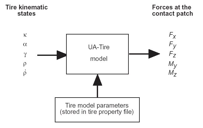
The UA-Tire model calculates the forces at the ground contact point as a function of the tire kinematic states, see Inputs and Output of the UA-Tire Model. A description of the inputs longitudinal slip κ, side slip α and camber angle  can be found in About Tire Kinematic and Force Outputs. The tire deflection
 and deflection velocity
 are determined using either a point follower or durability contact model. For more information, see Road Models. A description of outputs, longitudinal force Fx, lateral force Fy, normal force Fz, rolling resistance moment My and self aligning moment Mz is given in About Tire Kinematic and Force Outputs. The required tire model parameters are described in Tire Model Parameters.
can be found in About Tire Kinematic and Force Outputs. The tire deflectionand deflection velocityare determined using either a point follower or durability contact model. For more information, see Road Models. A description of outputs, longitudinal force Fx, lateral force Fy, normal force Fz, rolling resistance moment My and self aligning moment Mz is given in About Tire Kinematic and Force Outputs. The required tire model parameters are described in Tire Model Parameters.Inputs and Output of the UA-Tire Model
Definition of Tire Slip Quantities
Slip Quantities at Combined Cornering and Braking/Traction
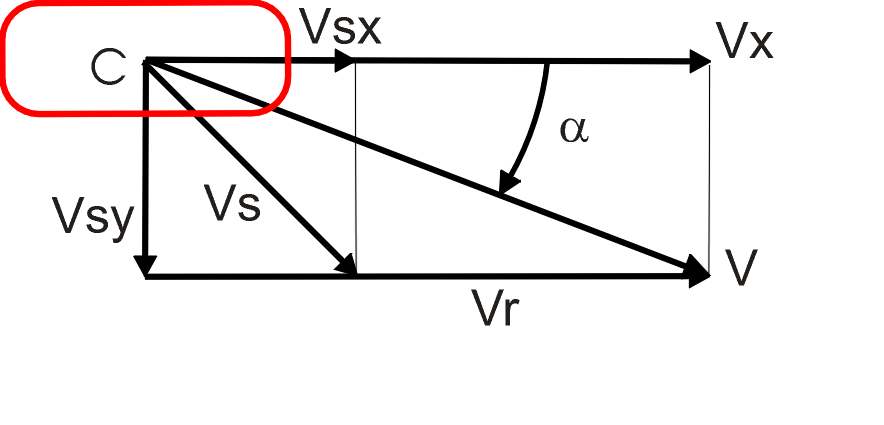
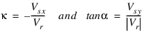
The longitudinal slip velocity Vsx in the SAE-axis system is defined using the longitudinal speed Vx, the wheel rotational velocity  , and the effective rolling radius Re:
, and the effective rolling radius Re: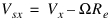
The lateral slip velocity is equal to the lateral speed in the contact point with respect to the road plane:

The practical slip quantities  (longitudinal slip) and
  (slip angle) are calculated with these slip velocities in the contact point:
(longitudinal slip) and (slip angle) are calculated with these slip velocities in the contact point: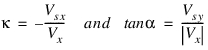
When the UA Tire is used for the force calculation the slip quantities during positive Vsx (driving) are defined as:
The rolling speed Vr is determined using the effective rolling radius Re:

Note that for realistic tire forces the slip angle  is limited to 45 degrees and the longitudinal slip Ss (=
  ) in between -1 (locked wheel) and 1.
is limited to 45 degrees and the longitudinal slip Ss (= ) in between -1 (locked wheel) and 1.Tire Model Parameters
Definition of Tire Parameters
Symbol: | Name in tire property file: | Units*: | Description: |
|---|---|---|---|
r1 | UNLOADED_RADIUS | L | Tire unloaded radius |
kz | VERTICAL_STIFFNESS | F/L | Vertical stiffness |
cz | VERTICAL_DAMPING | FT/L | Vertical damping |
Cr | ROLLING_RESISTANCE | L | Rolling resistance parameter |
Cs | CSLIP | F | Longitudinal slip stiffness,  |
 | CALPHA | F/A | Cornering stiffness,  |
 | CGAMMA | F/A | Camber stiffness,  |
UMIN | UMIN | - | Minimum friction coefficient (Sγ=1) |
UMAX | UMAX | - | Maximum friction coefficient (Ssγ=0) |
 | REL_LEN_LON | L | Relaxation length in longitudinal direction |
 | REL_LEN_LAT | L | Relaxation length in lateral direction |
* L=length, F=force, A=angle, T=time
Contact Methods
The UA-Tire model supports all Adams Tire contact methods.
■One Point Follower Contact, used by default for 2D Road, 3D Spline Road, OpenCRG Road and RGR Road.
■3D Equivalent Volume Contact, used by default for 3D Shell Road.
■3D Enveloping Contact, can be used with all road types when the keyword CONTACT_MODEL = '3D_ENVELOPING' is specified in the [MODEL] section of the tire property file.
The contact method supplies the tire model with the (effective) road height and road plane for the tire deflection/penetration calculation.
Force Evaluation in UA-Tire
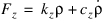
Normal Force
The normal force Fz is calculated assuming a linear spring (stiffness: kz ) and damper (damping constant cz ), so the next equation holds:
If the tire loses contact with the road, the tire deflection  and deflection velocity
  become zero so the resulting normal force Fz will also be zero. For very small positive tire deflections the value of the damping constant is reduced and care is taken to ensure that the normal force Fz will not become negative.
and deflection velocity become zero so the resulting normal force Fz will also be zero. For very small positive tire deflections the value of the damping constant is reduced and care is taken to ensure that the normal force Fz will not become negative.In stead of the linear vertical tire stiffness cz , also an arbitrary tire deflection - load curve can be defined in the tire property file in the section [DEFLECTION_LOAD_CURVE], see also the Property File Format Example. If a section called [DEFLECTION_LOAD_CURVE] exists, the load deflection datapoints with a cubic spline for inter- and extrapolation are used for the calculation of the vertical force of the tire. Note that you must specify VERTICAL_STIFFNESS in the tire property file but it does not play any role.
Slip Ratios
For the calculation of the slip forces and moments a number of slip ratios will be introduced:
Longitudinal Slip Ratio: Ss
The absolute value of longitudinal slip ratio, Ss, is defined as:

Where κ is limited to be within the range -1 to 1.
Lateral Slip Ratios: Sα , Sγ , Sαγ
The lateral slip ratio due to slip angle,  , is defined as:
, is defined as: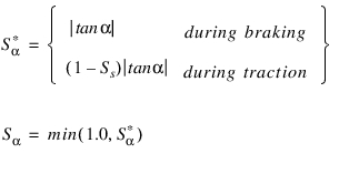
The lateral slip ratio due to inclination angle, Sγ, is defined as:

A combined lateral slip ratio due to slip and inclination angles, Sαγ, is defined as:
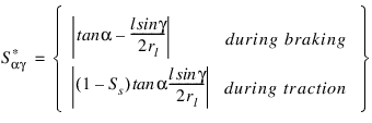
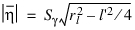
where  is the length of the contact patch.
is the length of the contact patch.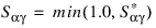
Comprehensive Slip Ratio: Ssαγ
A comprehensive slip ratio due to longitudinal slip, slip angle, and inclination angle may be defined as:
Friction Coefficient
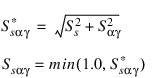
The resultant friction coefficient between the tire tread base and the terrain surface is determined as a function of the resultant slip ratio (Ssαγ) and friction parameters (Umax and Umin ). The friction parameters are experimentally obtained data representing the kinematic property between the surfaces of tire tread and the terrain.
A linear relationship between Ssαγ and  , the corresponding road-tire friction coefficient, is assumed. The figure below depicts this relationship.
, the corresponding road-tire friction coefficient, is assumed. The figure below depicts this relationship.Linear Tire-Terrain Friction Model
This can be analytically described as:
μ = Umax - (Umax - Umin) * Ssαγ
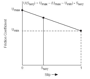
The friction circle concept allows for different values of longitudinal and lateral friction coefficients ( and
and  ) but limits the maximum value for both coefficients to
  . See the figure below.
and ) but limits the maximum value for both coefficients to . See the figure below.Friction Circle Concept
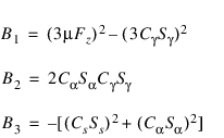
The relationship that defines the friction circle follows:
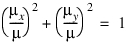
or  and
and 
and where:
Slip Forces and Moments
To compute longitudinal force, lateral force, and self-aligning torque in the SAE coordinate system, you must perform a test to determine the precise operating conditions. The conditions of interest are:
■Case 1: 
■Case 2:  and
and 
and ■Case 3:  and
and 
and ■Forces and moments at the contact point
The lateral force Fη can be decomposed into two components: Fηα and Fηγ. The two components are in the same direction if α * γ < 0 and in opposite direction if α * γ > 0.
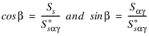
Case 1. αγ < 0
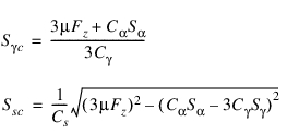
Before computing the longitudinal force, the lateral force, and the self-aligning torque, some slip parameters and a modified lateral friction coefficient should be determined. If a slip ratio due to the critical inclination angle is denoted by  , then it can be evaluated as:
, then it can be evaluated as:
If Ssc represents a slip ratio due to the critical (longitudinal) slip ratio, then it can be evaluated as:

If a slip ratio due to the critical slip angle is denoted by  , then it can be determined as:
, then it can be determined as: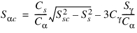
when  .
.
.The term critical stands for the maximum value which allows an elastic deformation of a tire during pure slip due to pure slip ratio, slip angle, or inclination angle. Whenever any slip ratio becomes greater than its corresponding critical value, an elastic deformation no longer exists, but instead complete sliding state represents the contact condition between the tire tread base and the terrain surface.
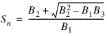
A nondimensional slip ratio Sn is determined as:

where
A nondimensional contact patch length is determined as:

A modified lateral friction coefficient  is evaluated as:
is evaluated as: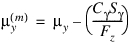
where  is the available friction as determined by the friction circle.
is the available friction as determined by the friction circle.To determine the longitudinal force, the lateral force, and the self-aligning torque, consider two subcases separately. The first case is for the elastic deformation state, while the other is for the complete sliding state without any elastic deformation of a tire. These two subcases are distinguished by slip ratios caused by the critical values of the slip ratio, the slip angle, and the inclination angle. Specifically, if all of slip ratios are smaller than those of their corresponding critical values, then there exists an elastic deformation state, otherwise there exists only complete sliding state between the tire tread base and the terrain surface.
(i) Elastic Deformation State: 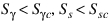 , and
, and 
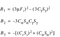
, and In the elastic deformation state, the longitudinal force Fξ, the lateral force Fη, and three components of the self-aligning torque are written as functions of the elastic stiffness and the slip ratio as well as the normal force and the friction coefficients, such as:
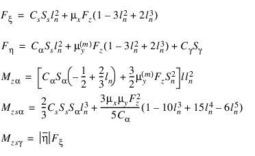
where
■ is the offset between the wheel plane center and the tire tread base.
is the offset between the wheel plane center and the tire tread base.■ is set to zero if it is negative.
is set to zero if it is negative.■ the length of the contact patch.
the length of the contact patch. is the portion of the self-aligning torque generated by the slip angle
  .
.  and
and  are other components of the self-aligning torque produced by the longitudinal force, which has an offset between the wheel center plane and the tire tread base, due to the slip angle
  and the inclination angle
  , respectively. The self-aligning torque Mz is determined as combinations of
  ,
,  and
and  .
.(ii) Complete Sliding State: 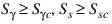 , and
, and 
, and In the complete sliding state, the longitudinal force, the lateral force, and three components of the self-aligning torque are determined as functions of the normal force and the friction coefficients without any elastic stiffness and slip ratio as:

Case 2:  and
and 
and As in Case 1, a slip ratio due to the critical value of the slip ratio can be obtained as:

A slip ratio due to the critical value of the slip angle can be found as:

when  .
.
.The nondimensional slip ratio Sn, is determined as:

where
The nondimensional contact patch length ln is found from the equation ln = 1 - Sn, and the modified lateral friction coefficient  is expressed as:
is expressed as: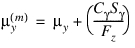
For the longitudinal force, the lateral force and the self-aligning torque two subcases should also be considered separately. A slip ratio due to the critical value of the inclination angle is not needed here since the required condition for Case 2,  , replaces the critical condition of the inclination angle.
, replaces the critical condition of the inclination angle.(i) Elastic Deformation State:  and
and 
and In the elastic deformation state:

(ii) Complete Sliding State:  and
and 
and 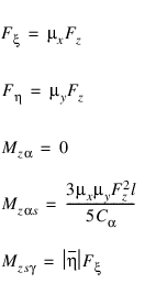
Case 3:  and
and 
and Similar to Cases 1 and 2, slip ratios due to the critical values of the inclination angle and the slip ratio are obtained as:
The nondimensional slip ratio Sn, is expressed as:
where

For the longitudinal force, the lateral force, and the self-aligning torque, two subcases should also be considered similar to Cases 1 and 2. A slip ratio due to the critical value of the slip angle is not needed here since the required condition for Case 3,  , replaces the critical condition of the slip angle.
, replaces the critical condition of the slip angle. (i) Elastic Deformation State:  and
and 
and In the elastic deformation state,  and
and  can be written:
and can be written: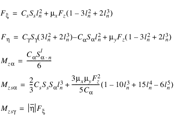
(ii) Complete Sliding State:  and
and 
and In the complete sliding state,  ,
,  ,
,  ,
,  , and
, and  can be determined by using:
, , , , and can be determined by using:
respectively. The longitudinal force  , the lateral force
  , and three components of the self-aligning torques,
  ,
,  , and
, and  , always have positive values, but they can be transformed to have positive or negative values depending on the slip ratio s, the slip angle
  , and the inclination angle
  in the SAE coordinate system.
, the lateral force , and three components of the self-aligning torques, , , and , always have positive values, but they can be transformed to have positive or negative values depending on the slip ratio s, the slip angle , and the inclination angle in the SAE coordinate system.Tire Forces and Moments in the SAE Coordinate System
For the general formulations of the longitudinal force Fx, lateral force Fy, and self-aligning torque Mz, in the SAE coordinate system, the three possible combinations of the slip ratio, the slip angle, and the inclination angle are also considered.
Longitudinal Force:
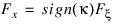 , for all cases
Lateral Force:
 , for cases 1 and 2
 , for case 3
Self-aligning Torque:

Rolling Resistance Moment:
My = -Cr Fz, for a forward rolling tire.
My = Cr Fz, for a backward rolling tire.
Transient Behavior in the UA-Tire Model
In the upper sections described force calculations are valid for the 'so-called' steady-state tire response, in other words tire dynamics is not taken into account. However, in general, the tire will be exposed to changes of input in terms of vertical load and longitudinal and lateral slip continuously.
For estimating transient tire behavior, a linear transient model is used as described in [1].
In the linear transient model the tire contact point S' is suspended to the wheel-rim plane with a longitudinal and lateral spring, with respectively stiffness's CFx and CFy. In the figure below a top view of the tire with the single contact point S' and the longitudinal (u) and lateral (v) carcass deflections is shown.
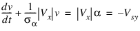
The contact point may move with respect to the wheel-rim plane and road. Movements relative to the road will result in tire-road interaction forces. Differences in slip velocities at point S and point S' will result in the tire carcass to deflect. The change of the longitudinal deflection u can be defined as:
and the lateral deflection v as:
For small values of slip the side force Fy can be calculated using the cornering stiffness CFα as follows:
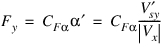
While the lateral force on the carcass reads:

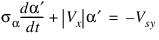
When introducing the lateral relaxation length σα as:

the differential equation for the lateral deflection can be written as follows:
For linear small slip we can define the practical slip quantity α' as:
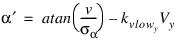
With α' the equation for the lateral deflection becomes:
Similar the differential equation for longitudinal direction with the longitudinal relaxation length σk can be derived:
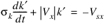
with the practical slip quantity 
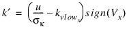
These practical slip quantities  and
and  are used instead of the usual
  and
and  definitions for steady-state tire behavior.
and are used instead of the usual and definitions for steady-state tire behavior.  and
and  optional the damping rates that can be applied to achieve more damping at low speeds (below the LOW_SPEED_THRESHOLD value). The LOW_SPEED_DAMPING parameter in the tire property file yields:
 = 100 ·
  = LOW_SPEED_DAMPING
The longitudinal and lateral relaxation length are read from the tire property file, see UA-Tire Property File Format Example.
Note that in transient mode the tire model is able to deal with zero speed (stand-still), because this linear transient model works with tire deflections instead of slip velocities. The effective lateral compliance of the tire at stand-still in transient mode is:

And similar in longitudinal direction the compliance is:

Note: | If the tire property file's REL_LEN_LON or REL_LEN_LAT = 0, then steady-state tire behavior is calculated. |
Reference
1. H.B. Pacejka, Tyre and Vehicle Dynamics, 2002, Butterworth-Heinemann, ISBN 0 7506 5141.
Operating Mode: USE_MODE
You can change the behavior of the tire model through the switch USE_MODE in the [MODEL] section of the tire property file.
■USE_MODE = 0: Steady-state forces and moments
The tire forces and moments react instantaneously to changes in the tire kinematic states.
■USE_MODE = 1: Transient tire behavior
The tire will have a lagged response because of the so-called relaxation length in both longitudinal and lateral direction. See Transient Behavior in the UA-Tire Model.
The effect of the relaxation lengths will be most pronounced at low forward velocity and/or high excitation frequencies.
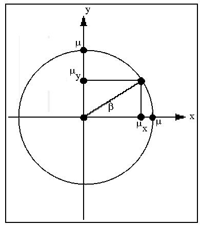
■USE_MODE = 2: Smoothing of forces and moments on startup of the simulation
When you indicate smoothing by setting the value of use mode in the tire property file, Adams Tire smooths initial transients in the tire force over the first 0.1 seconds of simulation. The longitudinal force, lateral force, and aligning torque are multiplied by a cubic step function of time. (See STEP in the Adams Solver online help.)
Longitudinal Force FLon = S*FLon
Lateral Force FLat = S*FLat
Aligning Torque Mz = S*Mz
Tire Carcass Shape
You can optionally supply a tire carcass cross-sectional shape in the tire property file in the [SHAPE] block. The 3D-durability, tire-to-road contact algorithm uses this information when calculating the tire-to-road volume of interference. If you omit the [SHAPE] block from a tire property file, the tire carcass cross-section defaults to the rectangle that the tire radius and width define.
You specify the tire carcass shape by entering points in fractions of the tire radius and width. Because Adams Tire assumes that the tire cross-section is symmetrical about the wheel plane, you only specify points for half the width of the tire. The following apply:
■For width, a value of zero (0) lies in the wheel center plane.
■For width, a value of one (1) lies in the plane of the side wall.
■For radius, a value of one (1) lies on the tread.
For example, suppose your tire has a radius of 300 mm and a width of 185 mm and that the tread is joined to the side wall with a fillet of 12.5 mm radius. The tread then begins to curve to meet the side wall at >+/- 80 mm from the wheel center plane. If you define the shape table using six points with four points along the fillet, the resulting table might look like the shape block that is at the end of the property format example (see SHAPE).
UA-Tire Property File Format Example
$--------------------------------------------------------MDI_HEADER
[MDI_HEADER]
FILE_TYPE = 'tir' FILE_VERSION = 2.0
FILE_FORMAT = 'ASCII'
(COMMENTS) {comment_string}
'Tire - XXXXXX'
'Pressure - XXXXXX'
'TestDate - XXXXXX'
'Test tire'
'New File Format v2.1'
$-------------------------------------------------------------units
[UNITS]
LENGTH = 'meter'
FORCE = 'newton'
ANGLE = 'rad'
MASS = 'kg'
TIME = 'sec'
$-------------------------------------------------------------model
[MODEL]
! use mode 1 2 3
! ------------------------------------------
! relaxation lengths X
! smoothing X
!
PROPERTY_FILE_FORMAT = 'UATIRE'
USE_MODE = 2
$-------------------------------------------------------dimension
[DIMENSION]
UNLOADED_RADIUS = 0.295
WIDTH = 0.195
ASPECT_RATIO = 0.55
$---------------------------------------------------------parameter
[PARAMETER]
VERTICAL_STIFFNESS = 190000
VERTICAL_DAMPING = 50
ROLLING_RESISTANCE = 0.003
CSLIP = 80000
CALPHA = 60000
CGAMMA = 3000
UMIN = 0.8
UMAX = 1.1
REL_LEN_LON = 0.6
REL_LEN_LAT = 0.5
$-------------------------------------------------------------shape
[SHAPE]
{radial width}
1.0 0.0
1.0 0.2
1.0 0.4
1.0 0.6
1.0 0.8
0.9 1.0
$---------------------------------------------------------load_curve
$ For a non-linear tire vertical stiffness (optional)
$ Maximum of 100 points
[DEFLECTION_LOAD_CURVE]
{pen fz}
0.000 0.0
0.001 212.0
0.002 428.0
0.003 648.0
0.005 1100.0
0.010 2300.0
0.020 5000.0
0.030 8100.0