Step Three - Adding Controls to the Adams Block Diagram
You will add controls to the Adams block diagrams by:
Starting Easy5
To start Easy5:
■Start Easy5 on your system from the directory that contains the file with the antenna example. This is the working directory that you created in Step One - Build the Adams Model.
The Easy5 main window appears.
Note: | The next two sections describe how to create a new Adams Interface block, and how to configure it to run different analyses. You should review these sections before proceeding to Constructing the Controls System Block Diagram where you will actually create a model (or load the existing example). |
Creating the Adams Interface Block
You create the Adams interface block by defining its component parts in the Add Components dialog box. After you define the component parts, you place the block in the work space area of the Easy5 main window.
To create the Adams interface block:
1. On left hand side of the Easy5 window, you should see a list of components (blocks) within Libraries and Groups.
If it's not already displayed, type Ctrl+A, and the Add Components window appears.
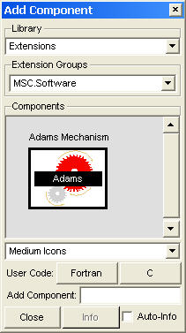
Figure 38 Add Components Window
2. Select a category for each of the component fields in the window.
■Under Library, select Extensions.
■Under Extension Groups, select Hexagon.
■Under Hexagon, select the Adams Mechanism block.
3. Move the cursor to the center of the Easy5 main window and click.
The Adams interface block appears. You build the controls block diagram by adding elements to this block.
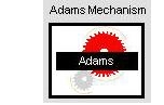
Figure 39 Adams Mechanism Block
Initializing and Configuring the Adams Interface Block
To initialize the Adams interface block:
1. Double-click the Adams interface block.
The Component Data Table appears as shown in Figure 40.
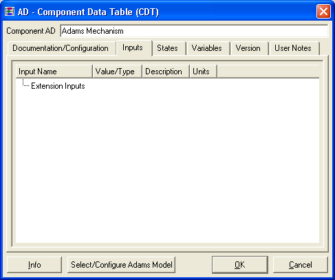
Figure 40 Component Data Table
2. Select Select/Configure Adams model in the lower left corner of the Component Data Table.
The Adams Interface dialog box appears as shown in Figure 41.
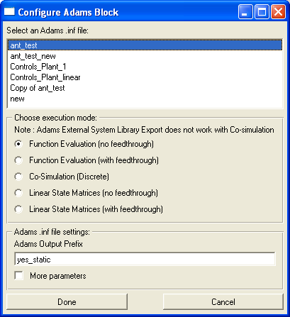
Figure 41 Adams Interface Dialog Box
3. Select ant_test.
4. Select Co-Simulation (Discrete).
Notes on the simulation options:
Options for Function Evaluation (1 and 2) are continuous simulation methods, integrating completely within Easy5. Option for co-simulation (3) is a discrete simulation method where Easy5 integrates the Easy5 model, and Adams integrates the Adams model, exchanging data at a specified communication interval.
Regarding Feedthrough: Feedthrough refers to whether the inputs directly affect the outputs (for example, forces directly affect accelerations), or not (for example, forces do not directly affect positions, velocities). In other words, if you've linearized a nonlinear Adams model and represented it as A, B, C, and D matrices and the matrix D is zero at all times, then there is no feed-through from the input variables to the output variables. If the matrix D is not zero at all times, then there is feed-through from the input variables to the output variables.
Options for Linear State Matrices (4 and 5) are linear methods that are solved completely within Easy5.
For information on choosing a simulation method, see the online help.
5. Select Done.
The Adams Interface dialog box closes, and the Component Data Table now looks like in Figure 42:

Figure 42 Component Data Table for Cosimulation
Tip: | For a description of the component inputs, outputs, and states, select the Info button |
Note: | You configure the Adams block the first time by reading in an .inf file. This defines the extension inputs, such as ADAMS_Animation_Mode, ADAMS_Solver, and so on. Subsequent reconfigurations of the block by reading in a new .inf file do not overwrite the existing setting. You can change the settings of the extension inputs at any time by manually resetting them before closing the Adams block CDT using the OK button. |
6. In the Component Data Table, in the Inputs tab, enter a value for the following input modes:
■For ADAMS_Animation_Mode, enter 1 to define interactive mode as the animation mode. For more details about animation modes, see the Adams Controls online help.
♦For ADAMS_Output_Interval (output rate interval), enter .001.
♦For Communication_Interval (communication rate interval between Adams and Easy5), enter 0.001. It should not be larger than the ADAMS_Output _Interval.
Note: | The ADAMS_Output _Interval in the Component Data Table determines the rate at which Adams Controls writes its result to file (and updates the animation, if in interactive mode). It is the interval at which the result is written to file once. It has the lower limit of Time Increment (see step 5), and works best if ADAMS_Output _Interval is a multiple of Time Increment for integration. The same rule applies to the Strip Chart output rate. |
■Alternatively, if you select Option 1 in step 4, the Component Data Table appears as follows:
♦In function evaluation mode, the communication interval option is not needed because the integrators determine the communication interval.
♦Leave Use_ADAMS_ICs at its default (1).
If the Use_ADAMS_ICs flag is set to 1, the model uses the Adams initial conditions.
If the flag is set to 0, the model relies on Easy5 to provide the initial conditions (for example, starting a simulation from the end of the last run simulation, which is stored in Easy5).
♦Set the parameters as shown in Figure 43.
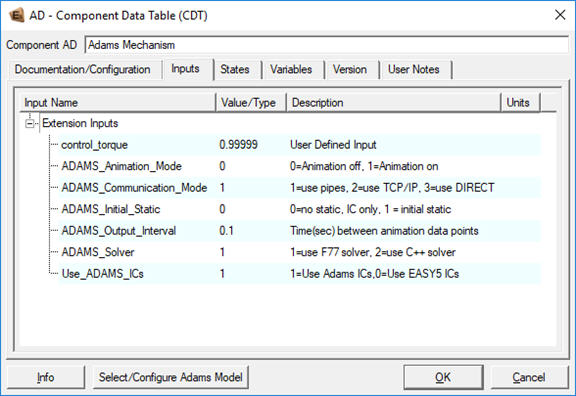
Figure 43 Component Data Table - Function Evaluation Mode
♦ADAMS_Solver has a default value of 1, which uses the Adams Solver (FORTRAN) for cosimulation or function evaluation. Setting this value to 2 allows you to use the Adams Solver (C++).
♦ADAMS_Communication_Mode has a default value of 1, which uses the pipes-based communication protocol for communication between Easy5 and Adams. Setting this value to 2 specifies that TCP/IP-based communication be used between the two products. For more information on TCP/IP-based communication, see TCP/IP Communication Mode in the Adams Controls help. Setting this to 3, enables DIRECT mode communication. Click on "Info" button in the Component Data Table to know more about this.
Constructing the Controls System Block Diagram
The completed block diagram is in the file, antenna.0.ezmf, in the examples directory. To save time, you can read in this diagram instead of building it.
Note: | Only one Adams block is allowed per Easy5 model. |
To construct the controls system block diagram:
1. Review the controls block diagram in Figure 44. Begin recreating the diagram with the blocks from the Add Components menu.
2. Place the Step Function Generator block in the diagram first.
3. Click on the Step Function Generator block using the middle mouse button.
The Component Data Table appears.
4. Set the step time (TO_SF) to 0.01 and the step value (STP_SF) to 0.3, and then select OK.
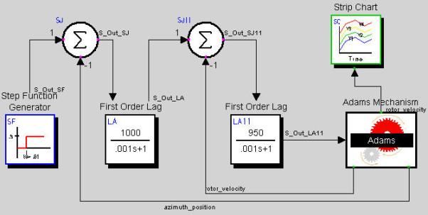
Figure 44 Controls Block Diagram
5. Connect the input blocks by clicking once on the First Order Lag block and then on the Adams Mechanism Block.
Easy5 labels this connection as S_Out_LA11.
6. Connect the output blocks in the diagram by clicking on the Adams Mechanism Block and then on the Summing Junction block. Be sure to connect the azimuth+position output to the first Summing Junction block (SJ) and the rotor_velocity output to the second Summing Junction block (SJ11).
7. Connect the Strip Chart to the Adams Mechanism Block.
Be sure to connect only the rotor_velocity output to the Strip Chart.
The rotor_velocity output corresponds to the rotor-velocity signal from the Adams Mechanism Block.
8. Click the Strip Chart using the middle mouse button to display the Component Data Table. Set the sample period TAU to .001, and then select OK.
Note: | You must edit the connection from the Adams Mechanism Block to the Strip Chart because Easy5 automatically connects the state vector from the Adams block to the display variable on the Strip Chart. |
9. From the File menu, select Save As, and then enter a file name for your controls block diagram.
You have now created the controls block diagram.