Step Four - Simulating the Model
You’ll simulate your mechanical model and controls system by:
Building the Executable
You must build an executable for your model before you execute a simulation in Easy5.
To build the executable:
■In Easy5, from the Build menu, select Create Executable.
After a few moments, Easy5 displays the message, Executable has been created, at the bottom of the main window.
You are now ready to execute the simulation.
Executing the Simulation
To execute the simulation from Easy5:
1. From the toolbar at the top of the Easy5 main window, point to Analysis, and then select Simulation.
The Simulation Data Form window appears.
2. Select the Plotting tab.
3. For plot variables, select Selected from the pull-down menu.
A Plot Specification Form appears where you define the variables that you want to plot after the simulation.
Note: | If you are using the completed block diagram from the file, antenna.0.ezmf, which was provided for you in the examples directory, you may find that the Plot Specification Form opens with information that is unnecessary for this tutorial. After removing this information, the Plot Specification Form should look like the shown in Figure 45. |
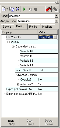
Figure 45 Plot Specification Form
4. Select the variables that you want to plot for the simulation.
For this tutorial, you will select three variables: rotor_velocity, azimuth_position, and S_Out_ LA11.
a. Under Dependent Variables, select the Variable #1 field.
Select the  icon next to the field. The Select Plot Variables select list appears.
icon next to the field. The Select Plot Variables select list appears.b. Expand the AD component, and then double-click rotor_velocity to select it.
The rotor_velocity component now appears as Variable #1 to be plotted.
■Repeat this procedure for the second and third variable. For the second variable, select azimuth_position, and for the third, select S_Out_ LA11 (the input to the Adams block  as indicated in Figure 44).
The finished Plot Specification Form should look like the one in Figure 46.
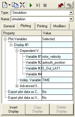
Figure 46 Plot Specification Form
5. Return to the General tab in the Simulation Data Form window, and then specify the following simulation parameters:
■For Start Time, enter 0.0.
■For Stop Time, enter .25.
■For Time Increment, enter .001.
■For Integration Method, enter BCS Gear.
6. Select the Play  tool to begin the simulation.
tool to begin the simulation. For more information about the simulation settings, see the Easy5 manual.
A new Adams View window appears and the analysis begins on the model specified in the Adams block. Adams View displays the analysis for you.
To run an interactive simulation:
1. As the simulation begins, arrange the windows so that you have a good vantage point to view the antenna model.
Note: | The Adams model is initialized to the current simulation time in Easy5. |
2. Start and pause the simulation by selecting Continue and Break on the interactive plot window.
Adams View accepts the control inputs from Easy5 and integrates the Adams model in response to them. At the same time, Adams provides the azimuthal position and rotor velocity information for Easy5 to integrate the Simulink model. The simulation process creates a closed loop in which the control inputs from Easy5 affect the Adams simulation, and the Adams outputs affect the control input levels. See Figure 2 for an illustration of the closed-loop simulation process.
Pausing and Stepping Through the Simulation
The interactive capabilities of Adams Controls let you pause the simulation in Easy5 and monitor the graphic results in Adams View. You can plot simulation results during pause mode.
To pause the simulation:
1. Select Break to pause the simulation at the next sample step.
You can use the interactive plot window (Figure 47) to pause the simulation, or you can single-step through the simulation. If you select Step, the simulation steps through one sample step (.001 seconds) of the interactive Strip Chart.
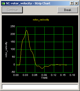
Figure 47 Interactive Plot Window
2. Now go back to Adams View. While the simulation is paused, you can change the orientation of the model with the View Manipulation Strip in the Main menu. These tools help you to look at the model from different vantage points.
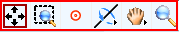
Figure 48 View Manipulation Strip
3. Once you have finished reorienting the model, select Continue to continue the simulation.
Adams View closes automatically after the simulation finishes.
Plotting from Easy5
Easy5 automatically displays the Plot window after running a simulation. By default, Easy5 displays the plot of the first variable you defined in the Plot Specification Form (see Figure 46). You can plot any data generated in Easy5 by selecting a variable from the Plot Selection Menu. In this tutorial, you’ll plot the curve for control torque.
To plot from Easy5:
■From the Plotter window, point to Displays, and then select the variable, S2 LA11, which is the control torque input to the Adams block from Easy5.
The Easy5 Plotter window displays the plot for control torque.
The Figure 49 shows how the plot should look. Notice that the control torque reaches a peak, and then settles down as the antenna accelerates. As the antenna gets close to its final position, the torque reverses direction to slow down the antenna. The antenna moves past its desired position, and then settles down to the point of zero error. At this point, the torque value is also zero.
To add labels to the plot:
1. At the bottom of the Plot Selection Menu, select Edit Display.
The Display Specification Form appears.
2. Enter the following labels:
■In the Plot Title text box, enter Adams Controls Torque Input from Easy5 to Adams.
■In the x-axis text box, enter time in seconds.
■In the y-axis text box, enter Control Torque, Newton-mm.
The labels you entered appear on the plot as shown in below.
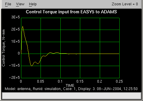
Figure 49 Plot of Control Torque Input
Plotting from Adams View
To plot from Adams View:
1. Display Adams View in a new system window and read in the command file, ant_test.cmd.
2. From the File menu, select Import.
The File Selection dialog box appears.
3. Select the following:
■For File Type, select Adams Results File.
■For Files to Read, select ant_test.res.
■For Model, select main_olt.
When you read in results files, be sure to include the model name because Adams View needs to associate the results data with a specific model.
Note: | You can plot any data from the simulation and rerun the animation from Adams View. |
4. From the Results tab, select Postprocessor.
Adams View launches Adams PostProcessor, a postprocessing tool that lets you view the results of the simulations you performed. Take a minute to familiarize yourself with Adams PostProcessor.
Figure 14 shows the Adams PostProcessor window
5. From the dashboard, set Source to Objects.
6. From the Model list, select .main_olt.
7. From the Filter list, select constraint.
8. From the Object list, select antenna_joint.
9. From the Characteristic list, select Element Torque.
10. From the Component list, select Y.
11. Select Add Curves.
Adams PostProcessor generates the curve.
To add labels to the plot:
1. In the treeview, navigate to the plot and select it.
2. In the Property Editor, in the Title text box, enter the name: Antenna Joint Peak Torque, Controlled.
The plot title appears above the plot.
Figure 41 illustrates how the curve should look. The curve shows the torque in the antenna joint from the azimuth control loop. You can use the information on the plot to help you determine how to modify the control system of the antenna model. For example, you can reduce the load in the antenna joint by decreasing the velocity gain of the azimuth controller at the expense of slowing the overall response of the controller. This is the type of trade-off between the mechanism design and the control design that you can analyze using Adams Controls.
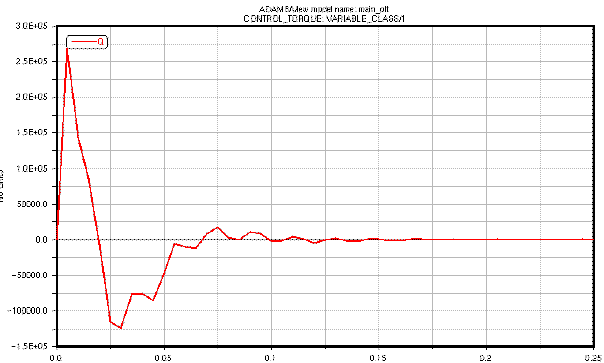
Figure 50 Adams Antenna Joint Peak Torque, Controlled