Splines
A spline creates a continuous function from a set of data points.
Learn about:
About Data Element Splines
A spline creates a continuous function from a set of data points. Splines are useful when you have test data or manufacturer specifications that specify the value of a function at several points. The spline can define a curve (two-dimensional, x, y) or a surface (three-dimensional, x, y, z).
You can use splines to create nonlinear functions for motions, forces, or other elements that use functions. In the case of a motion, the points define the displacement, velocity, or acceleration as a function of time, displacement, velocity, or another Adams quantity.
The Adams View spline element contains the x, y or x, y, z data points that you want to interpolate. To use the spline element, you must write a function expression that includes Adams spline functions (such as AKISPL or CUBSPL) or create a User-written subroutine that calls one of the spline utility subroutines (AKISPL or CUBSPL subroutine). The functions or subroutines interpolate the discrete data.
Ways to Create Splines
You can enter spline data into Adams View in several ways:
■Use the Spline Editor (see Create/Modify Spline dialog box help) to create a spline in Adams View. The Spline Editor provides you with a table for inputting values and a plotting window for viewing the results and the effects of different curve-fitting techniques.
■Use the general method to define spline data points by referencing either a file containing a set of points or results from a simulation. You can also enter numerical values directly. See Creating Splines Using the General Method.
■Import tabular data into Adams View and save it as a spline. For information on how to import test data as splines, see Import - Test Data.
■Use the data from a plot and save it as a spline. For more information, see Creating Splines from Curves in the Adams PostProcessor online help.
Note: | Large number of values pasted into user interface fields or data tables may result in application instability. MSC recommends users to enter no more than 1 million data points at a time. |
General Method for Creating Splines
Creating splines using the general method lets you define the data points of the spline using:
■File - The file is in RPC III, DAC, or user-defined format. The file contains x, y, and, optionally, z values that define the spline data points. You can specify that Adams View only use a particular named block or channel within the file. You can only enter time response data in RPC III and DAC files if you are using Adams Durability. For more information on using splines in Adams Durability, see Adams Durability online help.
Entering a user-defined file causes Adams Solver to call the User-written subroutine SPLINE_READ, which you must provide. For more on how to define a SPLINE using a user-defined file, see the example in SPLINE_READ of the Adams Solver Subroutines online help.
■Results of a simulation - You can also use the results of a Simulation as input to a spline by referencing Result set components. For more on result set components, see About Simulation Output.
■Numerical values directly input in the dialog box - You can directly input x, y, and, optionally, z values in the dialog box.
Curve-Fitting Techniques in Adams View
Adams View uses curve-fitting techniques to interpolate between data points to create a continuous function. If the spline data has one independent variable, Adams View uses a cubic polynomial to interpolate between points. If the spline data has two independent variables, Adams View first uses a cubic interpolation method to interpolate between points of the first independent variable and then uses a linear method to interpolate between curves of the second independent variable.
For information on the different spline functions that use these curve fitting techniques, see the definitions of the functions in Adams View Function Builder online help, and for a comparison of the different methods, refer to Spline Functions in the same help.
Creating Splines Using the Spline Editor
The Spline Editor provides a tabular or plot view of your spline data for editing and plotting. You can drag points on your spline plots and see the effect of different curve-fitting techniques on your spline. You can also select linear extrapolation and view its effect.
Using the Spline Editor, you can create a two- or three-dimensional splines.
Learn more:
General Procedures
Plotting a Spline:
Editing a Spline in a Table:
Displaying the Spline Editor and Setting the View
You can choose to view your spline as a plot or as a table in tabular format:
■Plot view
■Tabular view
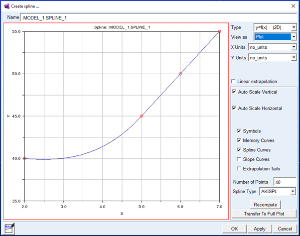
Spline Editor in Plot View
Viewing the spline as a plot lets you view the data in the spline as a curve and apply several operations on the curve, such as change the curve-fitting techniques being used to create the curve, view the results of linear extrapolation, or view the changes you made against the original spline values.
Spline Editor in Tabular View
Viewing a spline in tabular view gives you the most accuracy for setting the location of the spline data points. It also lets you quickly add points by inserting rows of data.
To display the Spline Editor:
■Click the Elements tab. From the Data Elements container, click the Spline tool .
.
. or
■(Classic interface) From the Build menu, point to Data Elements, point to Spline, and then select New.
To set the view of the Spline Editor:
■Set View As to either Tabular Data or Plot.
Setting Spline Units and Dimensions
You can specify the units that you want assigned for values in your spline in the Spline Editor. If you set the units for your data points, Adams View automatically performs any necessary unit conversions if you ever change your default modeling units.
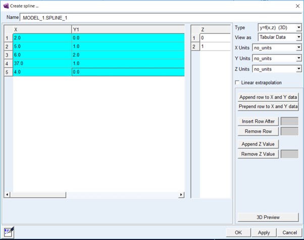
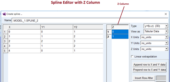
You can also select to create two- or three-dimensional splines. When you create a three-dimensional spline in tabular view, the Spline Editor displays a second column for adding z values as shown below. Note that you can view the z dimension in the 3D Spline Plot Viewer. You also need to recompute the spline in plot view to set a three-dimensional spline. (Learn about Viewing a Three-Dimensional Plot in the Spline Editor.)
To set units:
■Set X Units, Y Units, Z Units to the desired units. Select no_units if you do not want units associated with the values.
Note: | In the Adams View database and command language, units specification for splines can be done in either of two ways: via parameters "x_units", "y_units" and "z_units"; or by a single "units" parameter. If the Spline has this "units" parameter defined, it will be mapped to the Y Units field in this dialog. |
To specify two- or three-dimensional splines:
1. Set Type to either:
■y=f(x) (2D) to create or edit a two-dimensional, curve spline.
■y=f(x,z) (3D) to create or edit a three-dimensional, surface spline.
2. If you are in plot view to see the effect of the changes, select Recompute. Learn about Changing Plotting Methods and Recomputing the Plot.
Specifying Linear Extrapolation
Linear extrapolation extends the curve created from the spline values by estimating the values that follow from the spline values.
To specify linear extrapolation:
■Select Linear extrapolation.
To view the results of the linear extrapolation on the spline:
Learn about Curve-Fitting Techniques in Adams View.
Setting the View of the Spline Plot
When the Spline Editor is in plot view, there are several ways you can change the view of the spline plot, including viewing the slope of the curve, turning off the display of the data points that make up the spline, and more. Be default, Adams View displays a curve and hotpoints representing the spline data points. (Learn about Viewing a Three-Dimensional Plot in the Spline Editor.)
To view the curve that Adams View generates from the data points:
■Select Spline Curves.
If creating a 3D spline, you can view a 3D plot of the curves.
To view the slope (derivative) of a curve:
■Select Slope Curves.
To view the spline data points:
■Select Symbols.
You can edit the data points and, if creating a 3D spline, you can view a 3D plot of the points.
To retain the original curve as you edit the data points:
■Select Memory Curves.
To view the effect of linear extrapolation:
■Select Extrapolation Tails.
For more on setting up linear extrapolation, see Specifying Linear Extrapolation.
Viewing a Three-Dimensional Plot in the Spline Editor
In the Spline Editor, in either plot view or tabular view, you can display a three-dimensional (3D) plot of your spline. You must have set the type of the spline to 3D. (Learn about Setting Spline Units and Dimensions and Displaying the Spline Editor and Setting the View.)
In plot view, you can display two different 3D plots:
■Data Points - Using the 3D button next to Symbols displays the 3D spline using the raw data points (that is, the points represented by the curve symbols in the 2D plot). This is the same plot you see when you select to view a 3D plot in tabular view.
■Spline Representation - Using the 3D button next to Spline Curves displays a 3D plot using the spline representations Adams View generates from the raw data points. Each of the curves in the 2D plot represents one of the rows in the 3D preview plot.
In tabular view, to display a 3D plot of the data points:
■From the bottom right corner, select 3D Preview.
In plot view, to display a 3D plot of the data points:
■Next to Symbols, select 3D.
In plot view, to display a 3D plot of spline representations:
■Next to Spline Curves, select 3D.
To display the coordinates of a vertex on a 3D plot (called Probe mode):
1. Type a lowercase p.
2. Place the cursor over the vertex of interest.
The Spline Editor displays the coordinates (x, y, z values).
Editing Spline Plot Data
The left side of the Spline Editor in plot view displays a plot of the data points in the spline in plot view. Hotpoints appear on the curve in the plot window at each data point in the spline. You can drag the hotpoints to change the data point locations.
To edit data points:
1. Click the data point that you want to edit. Note that you must turn on the viewing of symbols.
Hotpoints appear at each data point.
2. Position the cursor on a hotpoint and drag the hotpoint to the desired location.
Changing Plotting Methods and Recomputing the Plot
By default in plot view, the Spline Editor displays a curve from your spline data points using 50 curve points and the Akima curve-fitting method. You can change the number of points and the method used to calculate the curve. You must recompute the spline to see the effect of these changes. As you recompute the spline, you can select to use the values stored for the spline in the modeling database or use the values as you've edited them.
To change the number of points used to display a curve:
■In the Points text box of the Spline Editor, enter the number of points.
Note: | Changing the number of points only changes the display of the curve, making it smoother or more coarse. It does not change the number of data points in the curve. |
To set the curve-fitting technique:
■Set Spline Type to either AKISPL or CUBSPL.
Learn about Curve-Fitting Techniques in Adams View.
To recompute the curve:
1. Select Recompute.
Adams View asks you if you want to use the current values for the spline or the ones stored in the modeling database.
2. Select one of the following:
■Yes to use the values in the database.
■No to use the edited values.
Transferring Plot to Adams PostProcessor
As you work on a spline in the Spline Editor, you can transfer its plot to Adams PostProcessor where you can save your plot and have it be accessible in Adams PostProcessor for such operations as creating reports. Note that any changes you make to the plot in Adams PostProcessor are not reflected in the actual spline object because you are editing the plot, not the spline data.
To transfer a spline plot:
1. In the lower right corner of the Spline Editor, select Transfer to Full Plot.
2. Display Adams PostProcessor to view the plot.
Working with Tables
The left side of the Spline Editor in tabular view displays the data points for the current spline. You can change any of the values in the cells of the Spline Editor and work with the cell much as you do in any spreadsheet editor.
To enter text in a cell:
1. Click the cell. The text cursor appears in the cell.
2. Type the text you want and press Enter.
To move to the next cell:
■Press Tab.
To move to the previous cell:
■Press Shift + Tab.
To move up to the previous row or down to the next row:
■Select the up or down arrow keys.
To cut or copy text in cells:
1. Select the text in the cell that you want to cut or copy.
2. Right-click the cell containing the text to be cut or copied, and then select Copy or Cut.
To paste text:
■Right-click the cell where you want to insert the text, and then select Paste.
To view the entire contents of a cell:
Often, information displayed in a cell of the Spline Editor is longer than the width of the cell. When this happens, Adams View displays the first portion of the information. In Linux, it also displays an arrow next to the cell to indicate that there is more information than can fit in the cell.
■Click in the cell. Adams View displays the last portion of the information in the cell.
To resize a column:
1. Point to the right border of the column heading that you want to resize. The cursor changes to a double-sided arrow.
2. Drag the cursor until the column is the desired size.
3. Release the mouse button.
Adding and Removing Rows
You can add rows to the X and Y table and to the Z table if you are creating a three-dimensional spline.
To add a row to the beginning of the X and Y table:
■Select Append row to X & Y data.
To add a row to the end of the X and Y table:
■Select Prepend row to X & Y data.
To add a row after a particular X and Y row:
■Enter a row number in the Insert Row After text box and select Insert Row After.
To add a row to the end of the Z table:
■Select Append Z Value.
To remove a row from either the X and Y or Z table:
■Enter the row number in the Remove Row text box and select Remove Row.
Creating Splines Using the General Method
To create a general spline using the general method:
1. Click the Elements tab. From the Data Elements container, click the Spline tool .
. or
(Classic interface) From the Build menu, point to Data Elements, point to Spline, and then select General.
The Data Element Create Spline dialog box appears.
2. Accept the default name or assign a new name.
3. Assign a unique ID number to the spline, if appropriate.
4. Add any comments about the spline that you want to enter to help you manage and identify it.
5. Set Linear Extrapolate to yes to extrapolate a spline by applying a linear function over the first or last two data points. By default, for user-defined files, Adams Solver extrapolates a spline that exceeds a defined range by applying a parabolic function over the first or last three data points. For RPC III or DAC files, the default method of extrapolation is zero-order (constant). Learn about spline extrapolation in Curve-Fitting Techniques in Adams View.
6. Depending on how you are creating the spline, enter or change the values in the dialog box as explained in the next table, and then select OK. See General Method for Creating Splines for available options.
To create a spline from: | Do the following: |
|---|---|
File | 1. Set the pull-down menu to File. 2. Enter the name of the file. 3. If desired, enter the block within the file from which you want Adams View to take the data. The block must be specifically named in the file. 4. Set the channel from which to take the data. This option is for use with time response data in RPC III files only. See Adams Durability online help. |
1. Set the pull-down menu to Result Set Component. 2. Select the result set components to be used for the x and y values. | |
Numerical input | 1. Set the pull-down menu to Numerical. 2. Enter the x, y, and, optionally, z values in the text boxes. Note the following: ■Specify at least four x and y values. The maximum number of x values, n, depends on whether you specify a single curve or a family of curves. ■Values must be constants; Adams Solver does not allow expressions. ■Values must be in increasing order: ■x1 < x2 < x3, and so on. |
Modifying Splines
The method you use to modify a spline (Spline Editor or general method) depends on the input to the spline.
■Numerical values or Result set components - If the input for the spline data points was numerical values or result set components, then when you select to modify the spline, Adams View displays the Spline Editor because it provides the most convenient method for directly editing values.
■File - If the method of input for the spline data points was a file, Adams View displays the Data Element Modify Spline dialog box, for you to change the file or interpolation method using the general method.
Note that because you do not always modify splines using the same method that you used to create them, you cannot change the input to the spline data points without first deleting the spline and making it again. For example, if you created a spline using the result set component TIME as the x values, and you want to change the spline to reference the result set component that defines the force on a part, you would have to delete the spline and create it again referencing the new component. In addition, if you defined spline data points using direct numerical values and you want to instead reference a file, you must delete the spline and make it again using the general method.
To modify a spline:
1. Click the Elements tab. From the Data Elements container, click the Spline tool .
. or
(Classic interface) From the Build menu, point to Data Elements, point to Spline, and then select Modify.
The Database Navigator appears.
2. Select a data element spline to modify.
The Spline Editor or Data Element Modify dialog box appears.
3. Follow the instructions in Creating Splines Using the Spline Editor or Creating Splines Using the General Method, as appropriate.
Tips and Cautions When Creating Splines
When selecting points to represent a curve or surface:
■Crowd points in regions with high rates of change.
■Spread out points in regions with slow rates of change.
The x and z data must cover the anticipated range of values. However, the following situations sometimes cause Adams Solver to evaluate a spline outside of its defined range:
■Adams Solver occasionally approximates partial derivatives using a finite differencing algorithm.
■Adams Solver occasionally attempts an iteration that moves the independent variable outside of its defined range. If this occurs, Adams Solver issues a warning message and extrapolates the four closest spline points. If the extrapolation is poor, Adams Solver can have difficulty reaching convergence, which may affect the results.
To avoid these problems, try to use real points, and extend spline values 10 percent beyond the total dynamic range.
Example of Using Splines
In this example, we use a spline to relate the force of a spring to its deformation. The values in the following Table show the relation of a force in a spring to its deformation.
Data Relating Spring Force to Spring Deflection Force
When the deflection is: | The force is: |
|---|---|
-0.33 | -38.5 |
-0.17 | -27.1 |
-0.09 | -15.0 |
0.0 | 0.0 |
0.10 | 10.0 |
0.25 | 30.0 |
0.40 | 43.5 |
0.70 | 67.4 |
Using this table, you can determine the force when deflection equals -0.33, and the force when deflection equals -0.17. You cannot, however, determine the force when the deflection is -0.25. To determine the force at any deflection value, Adams View creates a continuous function that relates deflection and force. The continuous approximation is then used to evaluate the value of the spring force at a deflection of -0.25. If you input two sets of values (x and y) using a spline data element, you can define the curve that the data represents.
You would then use the spline data element in a function or subroutine that uses cubic spline functions to fit a curve to the values. The curve allows Adams View to interpolate a value of y for any value of x.
Procedure
Briefly, the steps that you’d perform to use the spline data element to define the force deflections are:
1. Create the spline using the spline editor or the general method.
2. Build a simple nonlinear spring-damper, and then modify it to use the spline. To use the spline in the spring-damper definition, under Stiffness and Damping in the Spring-Damper Modify dialog box, change the stiffness coefficient to Spline: F= f(defo). Adams View builds a function expression for you, using AKISPL and modeled spring length as free length.
Note: | You can also use a single- or multi-component force to define the force deflections. In this case, you would select Custom as you create the force, and then modify the force by entering a function expression, such as: -akispl(dm(.model_1.PART_1.MAR_4,.model_1.ground.MAR_2) - 200.0, 0.0, .model_1.SPLINE_1) You can use the Function Builder for assistance in building the expression |
Linear Interpolation for 2D Splines
Adams View uses curve-fitting techniques (AKISPL and CUBSPL) to interpolate between data points to create a continuous function. If the spline data has one independent variable (2D spline), Adams View uses a cubic polynomial to interpolate between points. If the spline data has two independent variables (3D spline), Adams View first uses a cubic interpolation method to interpolate between points of the first independent variable and then uses a linear method to interpolate between curves of the second independent variable.
So, to perform the linear interpolation on a 2D spline, the workaround is to convert it into 3D spline.
The suggestion here is to edit the data such that the ‘Z’ which is the second independent variable will have all the values of first independent variable, ‘X’. The ‘Y’ will represent the dependent data in the following form: Y1-1,Y2-1,Y3-1 and so on.
To use this 3D spline, such that the function uses only second independent data, you should keep the first independent variable as zero; for example:
FUNCTION = AKISPL(0,time,SPLINE_1, 0)
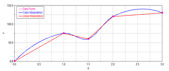
An example of linear interpolation is as follows:
■2D spline data:
0 0
1 75
1.5 60
2 120
3 130
■3D spline data of the above values in spline editor will looks like as follows:
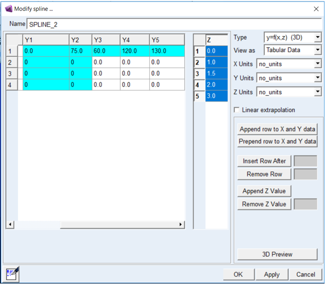
■Comparison between, the cubic and linear interpolated curve: