Expression Language Reference
This section explains how you can use expressions in Adams View to compute values or to parameterize your model. Parametrization lets you keep the associativity between model objects.
Learn more about:
Using Expressions in Adams View
You use expressions in Adams View in the expression mode of the Function Builder. Expressions are combinations of constants, operators, functions, and database object references, all enclosed in parentheses. In Adams View you can use expressions to specify parameter values, such as locations of markers or functions of motions.
Adams View uses expressions for two purposes:
■To compute values for you, such as when you are entering the radius of a cylinder and the value is not a simple number, but is the result of a mathematical computation. Instead of using a calculator to determine the actual number, you can enter the expression directly and let Adams View perform the computation for you.
■To parameterize your model. Expressions can contain references to other data values in Adams View. These expressions do not remain constant; Adams updates them each time the referenced data changes. Using expressions in this way allows you to make changes to one value and have this change propagate throughout your entire model. This is called parameterizing your model. If you are familiar with spreadsheets, this is identical to defining a cell as a function of another cell.
You construct Adams View expressions during model building. When Adams View reads an expression, it either evaluates it and stores the value in its database, or stores the expression itself.
Adams View includes variable objects intended for use with expressions. When creating an Adams View variable, you give it a name and a value. You can then include this variable, by name, in expressions; if you change the value of the variable, then Adams View updates the expression. In fact, any design variable or other object that changes will cause any expression that used it to re-evaluate. This allows you to parameterize your model using design variables. You can use such a parameterized model to do design studies, design of experiments, and optimizations.
Learn more (Expression Example).
Expression Syntax
The following sections introduce the elements you can use in expressions, and their proper syntax:
Data Types
All operands and the computed values of expressions are data that have a particular type. For information on operands, see Operands. There are five data types that Adams View expressions support: integer, real, string, matrix, and database object references. You can combine data of different types in an expression and Adams View coerces the data to the type needed to evaluate the expression. The following table lists the data types and their use.
Data type: | Use: |
|---|---|
Integer | Whole numbers in the range -maxint... +maxint, where maxint is machine dependent (usually around two billion) |
Real | Most numeric values |
String | Character strings of varying length |
Object | Database objects |
Matrix | One or two-dimensional collections of values of the same type, or one of the above types |
Operands
Operands allow you to indicate what you want to operate on. The kinds of operands allowed in Adams View expressions are:
Literal Constants
The first kind of operand is a literal constant value. Here are some examples of literal constant values:
Constant Value Examples
Constant value: | Example: |
|---|---|
Integer | 2 |
Real | 3.2 |
String | "x" |
Object | .model_1.part_5.marker_13 |
Matrix - Array of strings | {"x", "y"} |
Matrix - Array of reals | {[35,0], [3,6], [1,5]} |
Symbolic Constants
The second kind of operand in an Adams View expression is the symbolic constant. Adams View defines some frequently used constants with mnemonics, so you can use them easily and uniformly in your expressions. The table below lists the symbolic constants and their values.
Symbolic Constants
This constant: | Has this value: |
|---|---|
TRUE or YES or ON | 1 |
FALSE or NO or OFF | 0 |
PI |  = 3.1415 = 3.1415 |
HALF_PI |  |
THREE_HALVES_PI |  |
TWO_PI |  |
SIN45 |  |
SQRT2 |  |
RTOD |  |
DTOR |  |
VERSION | [Adams Release Version #] |
NONE | see explanation below |
NONE is a constant that behaves in a unique way. It can be coerced to any type and allows you to erase values from the database when used in certain contexts.
If used in arithmetic expressions, NONE equates to zero (10 + NONE is equal to 10). If used in string expressions, NONE is the empty string. Both of these facts can occasionally be useful in forcing type conversion of some value. For instance, the concatenation operator (//) takes a pair of strings and concatenates them into one: NONE // 2 forces the number 2 to become a character string, and NONE + "10" forces the string "10" to become the number 10.
The real power of the NONE constant is evident when it is used by itself in an expression, as shown by the following example.
Certain physical parameters of a model make a distinction between the value zero and a non-existent value. This is especially true during the solution of initial conditions of a model. Assume that you have an example model consisting of two parts joined together with a fixed joint. An initial conditions solution computes the initial velocities of these parts. If you assign one of the parts an explicit velocity, then Adams Solver sees that the two parts are constrained and sets the initial velocity of the other. This can only work if the second part has no velocity; if its velocity is undefined.
This command says that this part is not moving in the x direction, so its velocity is zero:
part modify rigid_body initial_velocity part=part_2 vx=0.0
The following command says that the velocity of this part is undefined, so you must examine other parts of the model to determine its initial velocity:
part modify rigid_body initial_velocity part=part_2 vx=(NONE)
In general, setting a parameter to NONE sets that parameter's value to non-existent.
Functions
A function is an operand that takes an argument list and computes a value based on the values contained in the list. Each argument is an expression that is evaluated and then given to the function. Common examples are SIN( ), SQRT( ), and ABS( ).
Adams View offers a wide variety of system-supplied design-time functions. For a complete list of design-time functions and how to use them, see Design-Time Functions.
The EVAL function is a special purpose design-time function that allows removal of subexpressions and dependencies from an expression. EVAL computes the value of its argument, without type coercion, and replaces itself with this value. This means that when you recall an expression from the database it never contains an EVAL function.
For example, if you create a variable whose value contains EVAL:
variable create variable=test real=(EVAL (2+2) / EVAL (2*3))
the database value for this variable is (4/6) and this is exactly the same as typing:
variable create variable=test real=(4/6)
There are two reasons to use the EVAL function:
■To eliminate costly recomputation of constant subexpressions. For example:
(EVAL(SQRT(2.2) + SIN(.55) + ATAN2(3,2)) + x)
is replaced by:
(57.8027713349 + x)
Note that the second expression is significantly faster, but lacks the readability of the first. It's very difficult to determine how Adams derived the constant 57.8027713349, and without some documentation you would never guess that it is actually the value SQRT(2.2) + SIN(.55) + ATAN(3,2).
Therefore, you use EVAL on subexpressions only when you can measure real time-savings, and document the resulting values thoroughly.
■To eliminate dependencies. You might encounter this problem when using loops:
for variable = XXX start=1 end=10
marker create marker=(UNIQUE_NAME("marker")) &
location=(EVAL(xxx)), 0, 0
end
If you don't use EVAL when defining the location of these markers, Adams parameterizes them to the variable xxx and moves them at each iteration of the loop. This would result in all of the markers being piled up at 10,0,0 after the loop terminated.
Database Objects and Their Component Values
Through expressions you can access most values stored in the Adams View database, regardless of whether you entered them through the command language or read them from a file. Adams View lets you access character strings, real numbers, integers, database objects, arrays, and boolean values.
To identify the database values you want to reference, use extensions of their Adams View hierarchical names by entering an entity's name and appending to it the name of the desired data field. The data an object owns is listed in the data dictionary. For more information on the data dictionary, see Getting Data Owned by an Object.
Accessing the Database
You can access the database to retrieve values from it to use in computing new values. To access the database, use the dot name notation. You have access to character strings, real numbers, integer numbers, database objects, arrays of real numbers and boolean values. In this release you do not have access to option values. The following sections provide more information on database access:
Reasons to access the Adams View database values include using the:
■Volume of one object to determine the mass of another.
■Locations of two coordinate systems to compute the orientation of a joint.
■Name of an object to derive new names for its children. For example, the name of a marker might be based upon the name of its parent part.
To identify the database values you want to reference, use extensions of their Adams View hierarchical names. This means you enter an entity's name and append the name of the desired data field to it. For example, to access the mass of the part named .model_1.part_1 you would enter,
.model_1.part_1.mass
Based on this, Adams View returns the real number value of the mass. We chose the name mass based on the full parameter name we used to set its value in the Adams View command language. That is:
part create rigid_body mass_properties part_name=.model_1.part_1 mass=1.0
When accessing the value of a design variable, you don't need the data field. For example, in the following commands, the expressions in the second and third command return the same value:
variable create variable_name=DV_1 real_value=100
variable create variable_name=DV_2 real_value=(DV_1.real_value)
variable create variable_name=DV_3 real_value=(DV_1)
Syntax
There is no specific command associated with database access. Adams View allows database access in any command parameter where it allows an expression. See Learning Function Builder Basics, for more information on using expressions in Adams View.
In the references given below, the dot (.) is used to separate components in the hierarchical name (just as it does in the current Adams View command language). You must enclose this name in parenthesis, to tell Adams View to recognize it as an expression. Note that enclosing a run-time function in parenthesis will not make it become an expression.
References can be either rooted or local. Rooted references have the following characteristics:
■Begin with a dot.
■Contain each specific component in the naming hierarchy (see the Rooted References table below).
■Parse faster than local references because they can be found by looking at the highest level of the database.
Rooted References
Database access: | Type: | Value retrieved: |
|---|---|---|
.some_model.some_part.mass | Real | Mass of a part |
.model_1.title | String | Title of model from .ADM file |
.model_1.circle_1.nsegs or .model_1.circle_1.segment_count | Integer | Number of sides of the circle |
.model_1.part_1.location | Array | Three-element location array |
.model_1.joint_1.i | Object | The i_marker used in joint_1 |
Local references have the following characteristics:
■Begin anywhere in the hierarchy before the field name.
■Contain only enough names to specify the object uniquely (see the Local References table below).
■Parse slower than rooted references because the entire database must be searched to find the specified object.
■All database names are case insensitive, as are all other parts of the Adams View command language.
Local References
Database access: | Type: | Value retrieved: |
|---|---|---|
some_part.mass | Real | The mass of some part |
part_1.name | String | The name of the part--"part_1" |
part_1.location[2] | Real | The second (y) element of location |
marker_1 | Object | The marker_1 database object |
coup.joint_name[indx].i_ marker_name.location[2] | Real | The second location of the i marker of the joint that is at the indxth position in the coupler named coup |
Syntax Examples
The following examples show the proper syntax for a variety of operations.
Setting a value:
part modify rigid_body mass_properties part=part_1 & mass=100!
Computing a mass:
part create rigid_body mass_properties part=part_2 & mass=(part_1.mass / 2.0)!
Computing a mass from a volume:
geometry create shape frustum frustum_name=fru_1 & top_radius=5 &
bottom_radius=10 &
length= 20part create rigid_body mass_properties part=part_2 &
mass=((fru_1.length * (fru_1.top_radius + fru_1.bottom_radius) / 2)**2 *PI)
Cautions
If you create a marker named "location" on part_1, then the following ambiguity can arise:
(part_1.location) meaning the marker named "location"
or
(part_1.location) meaning the location field of part_1
The first interpretation in the above example is how Adams would treat the expression. The algorithm used is:
1. Start at the database root and look for the first name, part_1 in this case.
2. Repeatedly look for a child object with the name following what you have already found, that is, location.
3. If you can't find a child object in the database, assume the name is a field and look it up.
In this particular case, either interpretation of expression (part_1.location) is valid in most contexts, but can produce very different results.
Aliases
You use aliases to reference fields on objects in the database. In addition to the parameters you see in commands and panels, there are many aliases for the components of aggregate fields, as listed in the data dictionary. (For more information on the data dictionary, see Getting Data Owned by an Object.) For instance, a marker location is a three-element array of real numbers. It has three aliases: loc_x for the first value, loc_y for the second, and loc_z for the third. In these cases you can enter the following:
marker create marker_name=new_marker location=(old_marker.loc_x), 1, 0
or
marker create marker_name=new_marker location=(old_marker.location[1]), 1, 0
When you use the alias (in the first example), the command executes faster, since no arithmetic has to be done to index the array element.
The following fields list some examples of aliases:
part.location
marker.location
marker.location
Indexed array: | Alias: |
|---|---|
alias location[1] | loc_x |
alias location[2] | loc_y |
alias location[3] | loc_z |
tire.inertia_moments
Indexed array: | Alias: |
|---|---|
alias inertia_moments[1] | ixx |
alias inertia_moments[2] | iyy |
For example, to obtain the x and y locations of Part_1, you could enter the following expression in the Function Builder:
({(.model_1.PART_1.location[1]),(.model_1.PART_1.loc_y)})
In this case, Adams View would return the location -50.0, -200.0.
Data Dictionary
The data dictionary lists the field names and the aliases associated with them, as they appear in expressions. You can access the data dictionary through the Function Builder, as explained in Getting Object Data.
Fields
Some database fields can't be parameterized. To determine if a specific field can be parameterized, try to parameterize it and examine the result. If the result is a constant value, then that field can't be parameterized. Adams View evaluates any expression that you enter in a field, and stores its result in the database.
Operators
You use operators to specify what you want to do to the operands. The operators table below lists the operators supported in Adams View expressions. They are listed by precedence, with grouping being the highest precedence operator.
Note: | Just as in FORTRAN, the exponentiation operator has precedence over the unary minus operator, and exponentiation associates from right to left |
Operators
Operator: | It means: |
|---|---|
( ) | Grouping |
[ ] | Indexing. Any matrix or multi-valued database object can be indexed. |
** | Exponentiation |
- | Unary minus = negation |
* / | Multiplication/division |
@ | Matrix multiplication |
+ - | Addition/subtraction |
< <= == > >= != | Relational. These operators allow you to compare objects of the same type. less than less than or equal to equal to greater than greater than or equal to not equal to |
! | Logical NOT. True if operand is false. |
&& | Logical AND. True if both operands are not zero. |
|| | Logical OR. True if either operand is not zero. |
// |
Real expressions containing integer division do not convert operands to real before division. This results in values as computed by Adams View, as shown in the example below,
1.0 + 1/3 = 1.0
not as evaluated in mixed mode arithmetic,
1.0 + 1/3 = 1.333
Also, in Adams View, 8/10 is equal to 0.
Whenever Adams View encounters a value of an inappropriate type in an expression, it attempts to coerce it to the proper type. If coercion fails, Adams View doesn't evaluate the expression and generates an error message. Operators determine coercion: the symbol + forces its operands to be numeric. Coercion is not order-dependent. The following table provides coercion examples:
Coercion Examples
Expression: | Result: | Description: |
|---|---|---|
2 + "2" | 4 | The character string is coerced to integer before arithmetic is performed. |
2 + 2 // 3 | "43" (2+2=4; 4//3=43) | Addition has higher precedence than concatenation; numbers are coerced to strings before concatenation. |
marker_1 + 1 | Error | Cannot convert database object to integer. |
Naming Conflicts
In Adams View you can create objects with names matching symbolic constants or matching the name of a data field of the created object. However, you should avoid doing this because it can make expressions confusing. If you must, however, Adams View has precedence rules for resolving these name conflicts. Consider the commands:
model create model=model_1
part create rigid_body name_and_position part_name=PI
part create rigid_body name_and_position part_name=part_1
marker create marker_name=.model_1.part_1.location
The name of part PI matches the symbolic constant PI, and the marker name .model_1.part_1.location matches the location field in the part named .model_1.part_1.
In the case of an object name being the same as a symbolic constant, using local names results in an error because Adams View looks for symbolic constants before database objects. Therefore, you need to use a rooted name to access the objects. For example:
(PI.mass) Returns errors--PI is interpreted as a symbolic constant
(.model_1.PI.mass) Returns the mass of part named PI
In the case of naming an object the same as a data field in the object being created, Adams View always returns the object instead of the field. For example, (part_1.location) returns the marker named location, not the location of the part.
Circular Expression Updating
Adams View monitors the values referenced by each expression. If you change a value used in an expression, Adams View immediately updates the expression.
When Adams View evaluates an expression, it can in turn cause the value of other expressions to change. Those expressions are re-evaluated to determine their new values. If an expression depends on its current value (either directly or indirectly), evaluation could continue endlessly. To avoid problems, Adams View only resolves such expressions one level deep.
For example, take the following expressions:
variable create variable_name=I integer_value=1
variable create variable_name=J integer_value=(I+1)
variable create variable_name=K integer_value=(J+2)
variable modify variable_name=I integer_value=(K+3)
When variable I is modified to reference K, Adams View determines that J depends on I and re-evaluates the value of J. Next, Adams View determines that K depends on J and re-evaluates the value of K. Finally, Adams View determines that I depends on K, but because I has already been updated, the re-evaluation is complete. Since variables might update in a different order, you might get varying results at different times.
It is possible to come up with expressions whose re-evaluation is unpredictable. Take, for example, the following commands:
variable modify variable_name=J integer_value=(K+M)
variable modify variable_name=K integer_value=(J+M)
variable modify variable_name=M integer_value=200
The third modify command changes the value of M, causing the values of J and K to be recomputed once. Their order of evaluation is unpredictable, hence the outcome of this computation is not defined and the results are not reliable. Use the EVAL function in these situations to eliminate circular references.
Location and Orientation
Adams View stores the positions (location and orientation) of objects in Cartesian/Euler coordinates, relative to the parent of the object containing the position (a marker's location is stored relative to the coordinate system of the part that owns the marker and all part locations are stored relative to the coordinate system of the model that owns the parts). When positions are specified with literal values, not expressions, Adams View computes database values using the current unit settings, and the default coordinate system (using the RELATIVE_TO parameter) before storing them.
When you use an expression to specify a position, Adams View stores the expression directly. Therefore, you must specify all position expressions consistent with how Adams View stores the positions. If you use an expression to specify the x, y, and z location of a marker, the coordinate system type must be Cartesian.
When you reference location and orientation values in an expression, Adams View uses their values exactly as they are stored. If you reference the location of a marker, its value is in Cartesian coordinates relative to its parent part.
You can use expressions to specify individual position components or an entire location or orientation. An example of using an expression to specify an individual component of a location is:
marker modify marker=marker_1 &
location=(2*CYL1.length),3,5.
An example of using an expression to specify an entire location is:
marker modify marker=marker_1 &
location=(LOC_RELATIVE_TO({2*cylinder_1.length,0,0},marker_1)).
Adams View supplies functions to specify positions parametrically. Some functions transform the locations and orientations from one coordinate system to another. Other functions allow you to parameterize your model similar to the more complex Adams View positioning features, such as RELATIVE_TO, ALONG_AXIS, and IN_PLANE. Certain functions, such as LOC_RELATIVE_TO, work independently of any local reference frame. If part, marker or other similar statements have a location or orientation parameter, the RELATIVE_TO can modify the values you supply.
For example, you might execute the following statements:
part create rigid_body name_and_location create part=part_1 location=1,1,1
part create rigid_body name_and_location create part=part_2 location=2,2,2
marker create marker=marker_2 location=0,0,0 relative_to=part_1
The above statements place marker_2 on part_1. In this case, the RELATIVE_TO parameter modifies the marker location you supplied.
When you use expressions for location or orientation, Adams View ignores the RELATIVE_TO parameter. In the following example, the RELATIVE_TO parameter plays no role for the location, but does apply to the orientation, since it doesn't have an expression:
marker create marker=marker_3
location=(LOC_RELATIVE_TO({0,0,0}, part_1)) &
orientation=90d,0,0
relative_to=(Part_2)
Locating Objects in Both Absolute and Relative Terms
To allow you flexibility in entering locations and orientations for objects, such as parts and markers, Adams View lets you specify a relative_to reference frame.
For example, you might know where a particular marker should be placed in absolute space, or you might know its location with respect to its part. In the first case, you could create the marker as follows:
marker create marker=.mod _1.part_1.marker_1
location=0,2,4 relative_to=.mod_1
In the second case, you would create the marker relative to part_1 to which it belongs:
marker create marker=.mod_1.part_1.marker_1
location=0,1,2 relative_to=.mod_1.part_1
This works for any reference frame (marker or part) that you might want. All you need to do is just create an object (markers are convenient) at the correct location and with the correct orientation, then specify new locations and orientations relative_to that object.
When defining the locations or orientation of objects using expressions, you cannot use a relative_to reference frame. With the above commands, Adams View transforms the information you supply for location and relative_to into a location relative to the part that owns the marker, and discards the values you entered. This loss of information is usually of no consequence, as you can easily reconstruct it (that is, you can set relative_to to anything you want and see the location or orientation expressed in that reference frame).
In both of the above cases, the value stored in the database for marker1's location is (0,1,2), and the value you supplied in the relative_to parameter is discarded. (Not only is the location stored relative to the part, it is also stored in Cartesian coordinates, so if you are using cylindrical or spherical coordinates on data entry, that information is also discarded.) Expressions are not this easily manipulated. The original information that you enter for a location expression must be maintained in the Adams View database to evaluate that expression.
This means that there are restrictions when you want to use expressions:
■You must set defaults units coordinate_system_type=cartesian.
■You must set defaults units orientation_type=body313.
■Any use of the relative_to parameter must be equivalent to system ground, as in relative_to=.mod_1.
Here is an example of a common mistake made with relative_to locations. In the example, marker_3 on part_3 must maintain its position in space but with respect to marker-2, which is on another part. It must be located at a position 5.0 units along the axis of marker_2 using LOC_ON_AXIS to compute the location of marker_3. See the diagram below.
marker create marker=.mod1.part_3.marker_3 & location=(LOC_ON_AXIS(marker_2, 5, "X"))
Note: | The text of the expression can break across lines. |
However, LOC_ON_AXIS places the marker one unit off in the direction (it is at a global position of (5,11,0) instead of the expected (4,11,0)). The LOC_ON_AXIS function computes a location in global space, so when you use the results of this function directly to locate a marker, the marker might not appear where you expect it. The solution is to use the results of the LOC_ON_AXIS function as an argument to the LOC_RELATIVE_TO function, which transforms the global result into that which the marker expects:
marker create marker=.mod1.part_3.marker_3 & location=
(LOC_RELATIVE_TO(LOC_ON_AXIS(marker_2, 5, "X"), .mod1))
Without this, the value is implicitly used relative to the owning part of the marker, therefore marker_3 appears in the wrong location.
Arrays
In the Adams View expression language, an array is a collection of values of the same scalar type.
Array Examples
Array: | Example: |
|---|---|
{1, 2, 3} | Array of integers |
{"red", "green", "blue"} | Array of character strings |
{.model_1, .model_1.part_1, part_3} | Array of objects |
{1.2, 3.4, 5.6} | Array of real numbers |
Arrays of real numbers can be multi-dimensional. This type of array is called a matrix and is explained in Matrices of Real Numbers.
When you create an array with elements of different type, Adams computes the element type to be the least common denominator, that is, something that works for all of the elements. Here are the rules for determining element type:
1. A string in an array forces all other elements to become strings:
{1, "red", marker_1} becomes {"1", "red", ".model_1.part_1.marker_1"}
2. If objects and numbers are mixed, the element type is string (since objects cannot be coerced to numbers and numbers cannot be coerced to objects):
{0, marker_1} becomes {"0", ".model_1.part_1.marker_1"}
3. Mixed integer and real numbers are all converted to real numbers:
{1, 2.5, 3} becomes {1.0, 2.5, 3.0}
The next sections explain the different types of arrays.
Empty Arrays
Adams View allows arrays to be empty. This is denoted by a pair of braces {}.
variable create variable=list real=({})
Note that this is distinctly different than the use of NONE; the value of the variable named list is an array that contains no values.
The following command creates a variable, named nothing, that contains an undefined value:
variable create variable=nothing real=(NONE)
The next section shows how such variables are different in a practical sense.
Concatenating Arrays
The concatenation operator works with arrays to attach one array to the end of another. The following sequence of commands creates a variable, named list, that contains the 11 values from 10 to 20 (the SERIES function would provide a more effective way of doing this):
variable create variable=list real=({})
for variable=value start=10 end=20
variable modify variable=list real=(EVAL(list // {value}))
end
The values resulting from the above example are: {10,11,12,13, ..... 20}.
If you create the initial value for list using NONE, as in the following example, you end up with a 12-element array containing an undefined value as the first element, followed by the values 10 through 20.
variable create variable=list real=(NONE)
The values resulting from the above example are: {0,10,11,12,13,..... 20}. In this case, the undefined value is 0.
Matrices of Real Numbers
Adams View stores multi-valued parameter values as real-valued two dimensional matrices.
The following sections provide more information regarding matrices of real numbers:
The way Adams View stores parameter values is important because it allows you to use matrix multiplication between any two real-valued arrays that have the proper shape. The following table shows how Adams View stores different parameter values.
How Multi-Valued Parameters are Stored
These parameter values: | Are stored as: | General math matrix syntax: |
|---|---|---|
Location and orientation |  |  |
Polyline location lists | Mx3 matrices |  |
Adams Solver dense-matrix data elements | MxN matrices |  |
All other real-valued matrices (such as spline x values or curve y-axis data) | 1xN matrices |  |
For example, if you've obtained a 3x3 transformation matrix via the TMAT function, you could use it to define a polyline, polyline_3. Here, polyline_3's location matrix has been parametrically defined as being dependent upon the array of polyline_2's location, and the angular orientation of marker_1.
Note: | @ is the matrix multiplication operator. |
Adams automatically converts a 1x1 matrix into a scalar if the context demands it, such as if the matrix is being passed as a parameter to a function that requires a scalar.
Entering Matrices in Expressions
When entering parameter values that are not expressions, simply enter the numbers one after another. For example, consider the polyline defined below by three points:
geometry create curve polyline polyline_name=polyline_1 &
location=({{1,2,3}, {4,5,6}, {7,8,9}})
or
geometry create curve polyline polyline_name=polyline_1 &
location=({[1,2,3], [4,5,6], [7,8,9]})
To enter a matrix in an expression, enclose the matrix in braces ({ }). Enter a multi-dimensional matrix in braces ({ }) or brackets ([ ]), depending on whether you want to enter column-major or row-major format, respectively. Each element inside a set of brackets denotes a row in the matrix. Each element inside a set of braces denotes a column in the matrix.
Creating Matrix Expressions of Various Dimensions
Adams matrix syntax: | General math matrix syntax: | Matrix dimension: |
|---|---|---|
 |  | 3 x 1  |
 |  | 3 x 2 |
{[11,12,13], [21,22,23], [31,32,33]} = {{11,21,31}, {12,22,32}, {13,23,33}} |  | 3 x 3 |
{[1,2,3]} = {{1}, {2}, {3}} | [1 2 3] | 1 x 3 |
Indexing
Indexing allows you to reference elements within a matrix, as shown in the table below:
Indexing in Adams
Adams index syntax: | Mathematical description: | Math result: | Adams result: |
|---|---|---|---|
 | Element in 2nd row, 1st column of the 3 x 1 matrix |  | 8 |
{[5,4,3]}[1,2] | Element in 1st row, 2nd column of the 1 x 3 matrix |  | 4 |
{[8,9], [5,6]}[2,1] | Element in 2nd row, 1st column of 2 x 2 matrix |  | 5 |
{1,2,3}[2] (see Note below) | Element in 2nd row, of the 3 x 1 matrix |  | 2 |
Note: | You can omit the second index when a matrix is 1xN (1 row) or Nx1 (1 column). |
You can use ranges of indexes to reference several elements of a matrix as shown in the table below:
Using Ranges of Indexes
Adams index syntax: | Mathematical description: | Math result: | Adams result: |
|---|---|---|---|
{[1,2,3], [4,5,6], [7,8,9]}[2:3,1:2] | 2nd to 3rd rows of the 1st to 2nd column |  | {[4,5], [7,8]} |
You can also extract a complete row of a matrix as shown in the table below:
Extracting a Complete Row
Adams index syntax: | Mathematical description: | Math result: | Adams result: |
|---|---|---|---|
{9,8,7}[2] | Element in 2nd row in 3 x 1 matrix |  | 8 |
{9,8,7}[2,1:1] | Element in 2nd row, 1st column of 3 x 1 matrix |  | 8 |
{9,8,7}[2,*] | Element in 2nd row, all columns of 3 x 1 matrix |  | 8 |
{[8,9], [5,6]} [1,1:2] | Element in 1st row, 1st to 2nd column of 2 x 2 matrix |  | {[8,9]} |
{[8,9], [5,6]}[1,*] | Element in 1st row, all columns of a 2 x 2 matrix |  | {[8,9]} |
Note: | * denotes all rows or all columns, depending on its placement. |
Adams View also allows you to extract a column of a matrix:
Extracting a Complete Column
Adams Index Syntax: | Mathematical Description: | Math Result: | Adams Result: |
|---|---|---|---|
{[8,9], [5,6]}[1:2,1] | Element in rows 1 to 2, 1st column of a 2 x 2 matrix |  | {8,5} |
{[8, 9], [5, 6]} [*,1] | Elements in all rows, 1st column of a 2 x 2 matrix |  | {8,5} |
{[1,2,3], [4,5,6], [7,8,9]} [*,1] | Elements in all rows, 1st column in a 3 x 3 matrix |  | {1,4,7} |
Note: | Indexing automatically converts any matrix with one element into a scalar. |
Database Fields Containing Multiple Data
Database fields containing more than one real number produce matrices. For fields containing location or orientation information, Adams View creates a 3 X 1 matrix:
marker create marker=marker_1 location=8,7,6
3x1 Matrix
Expression: | Result: |
|---|---|
marker_1.location | {8,7,6} |
marker_1.location [2] | 7 |
Adams View handles fields containing more than one location or orientation as 3xN matrices. For example, consider the three-point polyline defined below:
geometry create curve polyline polyline=polyline_1 loc=1,2,3, 4,5,6, 7,8,9
3xN Matrix
Expression: | Result: |
|---|---|
polyline_1.location | {{1,2,3}, {4,5,6}, {7,8,9}} or {[1,4,7], [2,5,8], [3,6,9]} |
polyline_1.location[*,2] | {4,5,6} |
polyline_1.location[2,3] | 8 |
Note the usefulness of this matrix format. If you have a 3 x 3 transformation matrix, T (T, as produced by the TMAT function), then post-multiplication by any matrix of locations or orientations produces a new matrix of the same shape. For example:
T @ marker_1.location (3x3 times 3x1) produces a 3x1 matrix.
T @ polyline_1.location (3x3 times 3xN) produces a 3xN matrix.
Using matrix composition with database objects, you can create a three-point polyline from marker locations:
geometry create curve polyline polyline=polyline_1 &
loc=({marker_1.location, {0,0,0}, marker_2.location})
The illustration below shows a three-point polyline:
For fields with multiple values, but with a single dimension, you create a 1 X N matrix:
data_element create spline spline=spline_1 x=1,2,3,4,5 y=2,3,4,5,6
1xN Matrix
Expression: | Result: |
|---|---|
spline_1.x | {[1,2,3,4,5]} |
spline.x[2] | 2 |
Note: | The same indexing operations that you can perform on database fields you can perform on a matrix with the same shape. |
Operators On Matrices
The following table lists the operators by precedence, from highest to lowest. All the standard binary operators are applicable to same-shape matrices (SSM), that is, matrices with the same row and column order, in a pair-wise fashion. Only one operator, the matrix multiplication operator (@), is not defined for SSM.
Operators on Matrices
Expression: | Result: | Comments: |
|---|---|---|
2 ** {0,1,2} {0,1,2,} ** 2 {1,2,3} ** {4,5,6} | (20,21,22) = {1,2,4} (02,12,22) = {0,1,4,} (14,25,36) = {1,32, 729} | Exponentiation |
-{0,1,2} | {0,-1,-2} | Negation |
{[1,2]} @ {3,4} |  | Matrix multiplication |
{1,2} @ {[3,4]} | 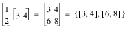 | Matrix multiplication |
2 * {0,1,2} {0,1,2,} * 2 {1,2,3} * {5,6,7} {[3,2]} * {[2,4]} | {0,2,4} {0,2,4} {5,12,21} {[6,8]} | Scalar multiplication Scalar multiplication Pairwise multiplication Pairwise multiplication |
2 / {1,2,3} {0,1,2} / 2 {1,2,3} / {5,6,7} | {2,1,0.667} {0,0.5,1} {0.2,0.333,0.429} | Division |
2 + {0,1,2} {0,1,2} + 2 {1,2,3} + {5,6,7} | {2,3,4} {2,3,4} {6,8,10} | Addition |
2 - {0,1,2} {0,1,2} - 2 {1,2,3} - {5,6,7} | {2,1,0} {-2,-1,0} {-4,-4,-4} | Subtraction |
2 == {0,1,2} {0,0,0} == 0 {1,2,3 }== {1,2,3} | {0,0,1} {1,1,1} {1,1,1} | Equality |
2 != {0,1,2} {0,0,0} != 0 {1,2,3} != {1,2,3} | {1,1,0} {0,0,0} {0,0,0} | Inequality |
2 <= {2,4,6} {2,4,6 } <= {3,4,5} | {1,1,1} {1,1,0} | Less than or equal (All other relational operators act similarly.) |
!{0,1,2} | {1,0,0} | Logical NOT |
2 && {0,1,2} {0,1,2} && 2 {1,2,3} && {5,6,7} | {0,1,1} {0,1,1} {1,1,1} | Logical AND |
2 || {0,1,2} {0,1,2 }|| 2 {1,2,3} || {5,6,7} | {1,1,1} {1,1,1} {1,1,1} | Logical OR |
Scalar Math on Matrices
All scalar math functions (including user-written functions) that take one or two real arguments and produce a real argument are applied to matrices in the same fashion as the unary and binary operators in the previous section:
Examples of Scalar Math on Matrices
Expression: | Result: |
|---|---|
SIN({1,2,3}) | {0.841471, 0.909297, 0.141120} |
ATAN2({1,2,3}, {3,2,1}) | {0.321751, 0.785398, 1.249046} |
ATAN2(3, {2,1}) | {0.982794, 1.249046} |
If you write a function ADD(x,y) that computes x+y, then, ADD(1,2) returns 3 and ADD({1,2,3}, {4,5,6}) returns {5,7,9}.
Units
Adams View allows you to assign units to numbers to explicitly define dimensions. For instance, the number 90 might be meaningful in the context of an angle only if it has units of degrees, while the number 3.14159 should probably have units of radians. Therefore, Adams View allows you to place labels on these values: (90d) or (3.14159r).
The following sections introduce you to unit sensitivity and unit labels:
Unit Sensitivity
The expressions you store in the database can be unit-sensitive, meaning that changing the current units results in a different value for the expression.
For example, if your model mass units are grams (g) and you have the part commands,
part_1 mass = 20
part_2 mass = (part_1.mass + 10)
then the mass of part_2 is 30 g.
Changing your model mass units to kilograms (kg) changes the mass of part_2 to 10.02 kg, because the mass of part_1 changed to 0.02 kg and part_2 = part_1 + 10. When this happens, Adams View issues the following message:
WARNING: The following values have changed due to unit sensitivity:
WARNING: .model_1.part_2.mass
Here's why: in the expression (part_1.mass + 10), 10 is a unitless constant. The value is 10 of whatever the context defines. When the units are grams, it is 10 grams; when the units are kilograms, it is 10 kilograms. On the other hand, the mass of part_1 is 20 grams (0.02 kg) independent of the current model units.
To make this expression non-unit-sensitive, simply add the unit label g after the 10.
part_2 mass=(part_1.mass + 10g)
Changing the model mass units, in this case from grams to kilograms, changes the mass of part_2 to 0.03 kg.
■In general, any expression that adds or subtracts a unitless constant to a unit-sensitive value is also unit-sensitive.
Symbolic constants such as PI and RTOD are unitless, as are generic reals and integers like 10 in the example above.
Expressions can also become unit-sensitive whenever involving any of the three trigonometric functions: SIN, COS, or TAN. When the angle parameter is a unitless constant, it is in the current angle units. If your angle units are radians, the expression calculates cosine of 45 radians:
(COS(45))
To make this expression non-unit-sensitive, simply add the unit label d after the 45, to calculate cosine of 45 degrees:
(COS(45d))
Unit Labels
To label an expression with units, you can use either simple unit labels or composed unit labels:
Simple Unit Labels
Simple unit labels are derived from the DEFAULTS UNITS command. Any unique abbreviation for a simple unit label is acceptable (radians = radian = radia = radi = rad = ra = r, since r doesn't conflict with any abbreviation for other units).
All of the simple unit labels, and their minimal abbreviations are listed in the table shown next, by their base units, in alphabetical order:
Simple Unit Labels and Their Minimal Abbreviations
Base units: | Simple unit labels: | Minimal abbreviations: |
|---|---|---|
Length | angstrom centimeter cm foot inch kilometer km m meter microinch micrometer mile mils millimeter mm nanometer yard | angs centimeter c f i kilometer km m met microi microm mile mils millimeter mm nanom y |
Angle | am angular_minutes angular_seconds as degree radian revolutions | am angular_m angular_s as d r re |
Mass | gram kg kilogram kpound_mass lbm megagram microgram milligram nanogram ounce_mass pound_mass slinch slug tonne us_ton | g kg kilogram kpound_m lbm meg microg millig nanog ounce_m pound_m sli sl t us_ |
Time | day hour microsecond millisecond minute ms nanosecond second | da ho micros millis min ms nanos s |
Force | centinewton dyne kg_force kilogram_force knewton kpound_force lbf meganewton micronewton millinewton nanonewton newton ounce_force poundal pound_force | ce dy kg_ kilogram_force kn kpound_f lbf megan micron millin nanon ne ounce_f pounda pound_f |
Frequency | hz radians/second | hz radians/sec |
Note: | For kilopound mass, kilonewton, and kilopound force, enter kpound_mass, knewton, and kpound_force, respectively |
There are three exceptions to unique aliases, as shown in the following table:
Exceptions to Aliases
Aliases: | Unit labels: |
|---|---|
d | Degrees, although it conflicts with dynes |
kg | Kilograms, although it conflicts with kg_force |
m | Meters, although it conflicts with mile, minute, ms, millisecond, and millinewton |
N | Newtons, although it conflicts with nanonewton |
r | Radians although it conflicts with revolutions |
The next table shows some examples of simple unit labels associated with a number within expressions:
Simple Unit Labels Associated with Numbers
Syntax: | Comment: |
|---|---|
1millimeter | Full label |
1.2 inch | Spaces are not significant |
24in | You can use abbreviations |
PI rad | You can apply unit labels to any expression, including symbolic constants |
Composed Unit Labels
Composed unit labels allow you to create aggregate units in a general way. You can do this by combining simple unit labels via operators. There are three operators you can use to compose aggregate units from existing simple units:
Operators Used in Composing Aggregate Units
Operator: | Notation: | Comment: |
|---|---|---|
exponentiation | ** | Right operand must be an integer: inch**2 |
multiplication | - or * | Foot-pound_f = foot*pound_f |
division | / |
The following table lists examples of composed unit labels:
Composed Unit Labels
3.3 (newton*meter) | Torque |
9.8 (meter/sec**2) | Composed acceleration |
PI (rad/sec**2) | Angular acceleration |
(SQRT(1)*3)(in - lbf) | Multiplication with a dash '-' |
1.2 (inch / (sec*deg)) | ERROR! no parenthesis allowed inside composed units |
1.2 (inch / sec / deg) | Correct way to compose this |
Note: | To eliminate ambiguity, always enclose unit labels in parentheses. In general, if you see units associated with numbers produced by the list_info command in a command file or anywhere else, you can take that units string and use it in an expression. |