Overview

When working with flexible bodies, you will often find that Adams standard forces and torques are inefficient for defining distributed loads acting on a large number of nodes. Adams Flex, therefore, provides you with methods for modeling distributed loads and predeformed flexible bodies.

Select a topic for scenarios for when modeling distributed loads and preloaded flexible bodies is helpful and an introduction of the Adams modal force (MFORCE), which you can use to define distributed applied loads. There are also tutorials so you can try out these features, and explanations of how to create a loadcase file.

For general information on creating and managing MFORCEs and preloads in Adams View and Adams Solver, see:

To illustrate the ways in which you model applied loads and preloads, we've provided two user scenarios. One is an example of a distributed applied load and the other is an example of a preloaded flexible body.

A flexible component that undergoes a change in temperature expands or contracts. A finite element analysis (FEA) program determines the associated thermal loads based on the material properties of the component. Adams View, however, does not possess finite element capabilities and, therefore, cannot determine these loads. The thermal load has components acting on each node of the finite element model. Introducing this load to Adams as a collection of point forces is impractical and inefficient.

The alternative is to express the load in terms of the modal degrees of freedom (DOF) rather than nodal DOF. After the FEA program prepares a component mode description of the flexible component for Adams, it takes any user-defined loadcases, such as the thermal loadcase, and transforms them from nodal DOFs to modal DOFs by projecting the load vector on the mode shapes. It then exports the load to Adams in the form of modal loads, one set of modal loads for each user-defined loadcase.

In Adams Flex, you can scale the modal loads corresponding to a particular loadcase and combine them with other loadcases. You can make the scale factor a function of time or of system response. In the example of a flexible component undergoing temperature change, you might scale the thermal load as a function of simulation time, of the velocity of the object, or of the proximity to a heat-source, and others.

Other sources of distributed loads include the aerodynamic lift on a flexible airplane wing or the combustion force on the dome of a piston. You can also model these distributed loads using an FEA program and export them to Adams Flex, where you can combine them in many different ways.

For a more detailed technical description, see MFORCE in the Adams Solver Help.

An automobile tire has highly nonlinear material properties and experiences large nonlinear deformations. For these reasons, you would not normally consider modeling a modal representation of the tire in Adams Flex. However, in certain Adams analyses, you can safely assume that the deformations of the tire will remain within a small range around a fixed operating point and a linearization of the tire about this operating point would yield a useful modal representation of the tire. A nonlinear finite element model of the tire is brought to this operating point by applying a combination of a contact force, inflation pressure, and a spin. The tire is linearized at the operating point and the modes are extracted and exported to Adams Flex.

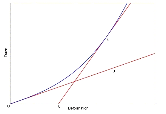
The figure below illustrates the process described above. An undeformed tire is defined by operating point O. As it deforms, it is brought through a nonlinear path to a deformed state A. A linearized description of the tire at O, such as the one earlier versions of Adams Flex would have been limited to, would incorrectly predict a deformed operating point at B rather than A. Using the preload support in Adams Flex, it is now possible to define an alternative linearized description of the tire, at A rather than O. This Adams flexible body might be quite suitable for an analysis of a tire near operating point A. A limited range of validity of the linearized representation must still be observed. For example, fully unloading the Adams flexible body that represents A would bring it to operating point C, which is not correct.

You may also want to define predeformed flexible bodies when working with models of linear elastic components. For example, it can be more convenient to define a valve-train model when a valve-spring has been predeformed so that its size matches its configuration when the components of the model have been assembled.

To further distinguish the two forms of loads, consider that preloads have been applied to the flexible component in the FEA program before it is exported to Adams. The applied distributed loads, while formulated in the FEA program, are not applied in the FEA program. Preloads become a permanent part of the flexible body description and cannot be deactivated. Distributed applied loads are exported to Adams where you can scale, combine, and apply them to the flexible body as necessary. You export both types of loads through the Modal Neutral File (MNF).

You can review modal forces on flexible bodies in Adams PostProcessor as:

No matter what form, the modal force results are presented with respect to the flexible body’s local part reference frame. This is unlike most other Adams force elements that are plotted with respect to the ground coordinate system, by default. For a detailed overview of modal forces and a tutorial that steps you through an example of creating a modal force, see Modeling Distributed Loads and Predeformed Flexible Bodies.

The following tutorials let you try out the features helpful when modeling distributed loads and preloaded flexible bodies.

The MFORCE distributed load and modal preloads capabilities assume that additional values are stored in the flexible body's Modal Neutral File (MNF). Currently, few finite element analysis (FEA) programs that support Adams Flex provide this capability. As an interim solution, MSC Software has developed a tool, mnfload, which adds applied modal loads and preloads to existing MNFs. Support for these capabilities from FEA programs will be announced as it becomes available.

Learn more on how to use mnfload:

You invoke mnfload from the command line using the command:

where:

The variable loadfile in the command to invoke mnfload is an ASCII file containing a concatenation of loadcases. Each loadcase starts with the identifier line:

where:

Note that there can only be one preload and it must be a balanced load. There can be no global resultant load components. In other words, the preload must be an internal load.

Each loadcase identifier line is followed by lines defining either nodal forces and torques or modal loads. When defining the nodal force, the format of the lines are:

where:

When defining a modal load in modal coordinates the format of the load lines is:

where:

The following file defines three loadcases:

Note that the preload is invalid unless nodes 1000 and 1001 have the same y and z coordinates; otherwise this would not be a balanced load.