LINEAR
The LINEAR command is divided into the following sections:
1. General
You can use the LINEAR command to linearize Adams models. Linearized Adams models can be represented by complex valued eigendata (eigenvalues, mode shapes) or by a state-space representation in the form of real-valued state matrices. Two state-space representations are possible, the ABCD standard representation and the MKB Nastran representation. Moreover, the LINEAR command can be used to export the linearized Adams model into an equivalent Nastran bulk data deck.
Adams Solver (C++) uses a state-of-the-art condensation scheme to reduce an Adams model to a minimal linear form for efficient solution. (For more information, see On an approach for the linearization of the Differential Algebraic Equations of Multi-body Dynamic, D. Negrut and J. L. Ortiz. Fifth ASME International Conference on Multibody Systems, Nonlinear Dynamics and Control, ASME 2005.)
The LINEAR command has four main options designed to provide important insight into the dynamic behavior of the model. For instance, the LINEAR/EIGENSOL option can be used to assess the stability of the model. Stability properties of the model have a direct relationship to the real part of the complex eigenvalues. Eigenvalues with positive real parts represent unstable modes of the system, while those with negative real parts represent stable modes. If bounded inputs to the system cause excitation of an unstable mode, the system produces an unbounded response. On the other hand, bounded excitation of a stable mode results in a bounded response. Eigenvalues computed by Adams Solver (C++) can be plotted on a real-imaginary plot and the mode shapes can be animated using Adams View. In addition to verifying stability, eigendata is used for validating implementation of models with eigendata from other modeling approaches or experimental data. This is especially true if an elastic or control sub-system model has been implemented in Adams Solver (C++). If you issue the LINEAR/EIGENSOL option, Adams Solver (C++) computes the model eigendata and reports the model eigenvalues to the workstation screen. If the results outputs are enabled, eigendata is also written into the results (.res) file, and may be taken to Adams for further processing.
Important: | The LINEAR/EIGENSOL option RESULTS statement should have the XRF option. Otherwise the eigendata is not written into the results file and this cannot be postprocessed in Adams View or PPT. |
Both the LINEAR/STATEMAT and the LINEAR/MKB options output a state-space representation in a form suitable for importation into matrix manipulation and control design packages such as MATRIXx and MATLAB (for more information see the Xmath Basics Guide, 1996, Integrated Systems Inc., Santa Clara, CA and Matlab User's Guide, The MathWorks Inc., Natick, Massachusetts). A state-space model representation is suitable for obtaining frequency response of the Adams model, verifying model control properties (controllability and observability), and designing feedback controllers for Adams models. If you issue the LINEAR/STATEMAT or LINEAR/MKB command, Adams Solver (C++) computes the state matrices for the model and writes them to a user-specified file or files. If enabled, state matrices are also written out to the Results file.
Option LINEAR/EXPORT is used to export the linearized model into an equivalent Nastran model. Using this option, Adams Solver (C++) creates an ASCII file containing a Nastran bulk data deck. Two sub options are available: a "closedbox" sub option equivalent to a state space representation, and a "openbox" sub option in which an element-to-element export is performed. Using the "openbox" sub option, rigid Adams PARTS are exported as CONM2 cards, Adams JOINTS are exported as RJOINT cards or sets of MPC cards and so on. Both the "closedbox" and "openbox" sub options honor a configuration file which is used to fine tune the exporting process. The configuration file can be used to custom the exported model. See below for current limitations of the LINEAR/EXPORT option.
2. Definition
The LINEAR command linearizes the nonlinear system equations of motion and provides four basic capabilities: an eigensolution, a standard state-space matrix calculation, a Nastran-specific state space calculation, and an export to a Nastran bulk data deck.
The eigensolution option determines natural frequencies and mode shapes while the state space calculations compute the linear state space matrices that describe the linearized mechanical system.
You may issue this command following initial conditions, a static or a transient analysis. Depending on the options you specify, the results of the command are reported on the screen and written to the Message file, the Results file, and, if required, the user-specified files.
The LINEAR/EXPORT option has been modified to support all types of operating points (static or dynamic). However, matching eigenvalues with Nastran can be obtained using static operating points only. Kinematic models (zero degrees of freedom) can only be exported using the OPENBOX option.
For theoretical details on the linearization algorithm, see the white paper in Simcompanion Article KB8016460.
3. Format
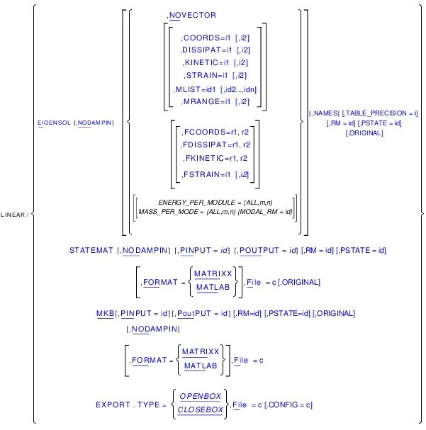
4. Arguments
CONFIG=c | Specifies a file name from which Adams Solver (C++) reads configuration directives to customize the export process to a Nastran bulk data deck. If no configuration file is specified, Adams Solver (C++) will use default configuration parameters. See below for the syntax of the configuration file. Range: Valid file name. Type: Optional with EXPORT. |
COORDS=i1[,i2] | Specifies that a table of coordinates for mode numbers in the range i1 to i2 be computed and output. If i2 is not specified, Adams Solver (C++) produces the table of coordinates for mode number i1 only. Range: i1 > 1, i2 > i1 Type: Optional with EIGENSOL; mutually exclusive with NOVECTOR |
DISSIPAT=i1[,i2] | Specifies that a table of dissipative power distribution for mode numbers in the range i1 to i2 be computed and output. If i2 is not specified, Adams Solver (C++) produces the table of dissipative power distribution for mode number i1 only. Range: i1 > 1, i2 > i1 Type: Optional with EIGENSOL; mutually exclusive with NOVECTOR |
EIGENSOL | Specifies that Adams Solver (C++) performs an eigenanalysis of the Adams model. Type: Optional (either EIGENSOL, MKB, STATEMAT or EXPORT is required) |
ENERGY_PER_MODE={ALL m,n} | Specify Adams Solver to compute energies for each mode in the eigenanalysis. m,n specifies the mode range to report the energies per mode. All is used for all modes. Percentages reported in table are computed with respect to the requested mode range. |
EXPORT | Specifies that Adams Solver (C++) performs a Nastran bulk data deck export. Type: Optional (either EIGENSOL, MKB, STATEMAT or EXPORT is required) |
FILE=c | If using the STATEMAT or MKB options, specifies a file name to which Adams Solver (C++) writes the state matrices. If the output is in the MATRIXX format, all matrices are written to this file. For the MATLAB format, the file name is used as a base name. Each matrix is written to a separate file, whose name Adams Solver (C++) automatically constructs by appending the matrix name to the user-specified base name. If using the EXPORT option, specifies a file prefix for the bulk data deck to which Adams Solver (C++) writes the exported data. Range: Valid file name up to 76 characters Type: Required with MKB or STATEMAT or EXPORT |
 | Specifies the name of the software in whose input format Adams Solver (C++) is to output the state matrices. Presently, two software formats are supported: MATRIXX (FSAVE format) and MATLAB (ASCII flat file format). This argument is a qualifier for the MKB or STATEMAT option. Type: Optional with MKB or STATEMAT Default: MATRIXX |
KINETIC=i1[,i2] | Specifies that a table of kinetic energy distribution for mode numbers in the range i1 to i2 be computed and output. If i2 is not specified, Adams Solver (C++) produces the table of kinetic energy distribution for mode number i1 only. Range: i1 > 1, i2 > i1 Type: Optional with EIGENSOL; mutually exclusive with NOVECTOR |
MASS_PER_MODE={ALL m,n} [,MODAL_RM=id] | Specify Adams Solver to compute effective mass and modal participation factors for each mode in the eigenanalysis. m,n specifies the mode range to report the effective mass and participation factors. ALL is for all modes. Percentages reported in table are computed with respect to the requested mode range. Optionally, a marker id can be specified as the reference frame for computing effective mass. The default is the global frame. |
MKB | Specifies that Adams Solver (C++) calculates the M, K, B, C and D matrices for the Adams model. These matrices are used as inputs to a MSC.NASTRAN model. Type: Optional (either EIGENSOL, MKB, STATEMAT or EXPORT is required) |
MLIST=id1[,id2..., idn] | Specifies that a table of marker mode for mode numbers in the MRANGE be computed and output. Specify the marker IDs: id1, id2 ..., idn. Range: i1 > 1, i2 > i1 Type: Optional with EIGENSOL; mutually exclusive with NOVECTOR. Required with MRANGE. |
MRANGE=i1[,i2] | Specifies that a table of marker mode for mode numbers in the range i1 to i2 be computed and output. If i2 is not specified, Adams Solver (C++) produces the table of marker mode for mode number i1 only. Range: i1 > 1, i2 > i1 Type: Optional with EIGENSOL; mutually exclusive with NOVECTOR. Required with MLIST. |
FCOORDS=r1, r2 | Specifies that a table of coordinates for modes with frequencies in the range r1 to r2 be computed and output. If a mode has a real-only frequency, the mode is ignored. If a mode has a complex eigenvalue, the table will be output only if the absolute value of the imaginary part is in the specified range. Range: r2 > r1 > 0. Type: Optional with EIGENSOL; mutually exclusive with NOVECTOR and COORDS. |
FKINETIC=r1, r2 | Specifies that a table of kinetic energy distribution for modes with frequencies in the range r1 to r2 be computed and output. If a mode has a real-only frequency, the mode is ignored. If a mode has a complex eigenvalue, the table will be output only if the absolute value of the imaginary part is in the specified range. Range: r2 > r1 > 0. Type: Optional with EIGENSOL; mutually exclusive with NOVECTOR and KINETIC. |
FSTRAIN=r1, r2 | Specifies that a table of strain energy distribution for modes with frequencies in the range r1 to r2 be computed and output. If a mode has a real-only frequency, the mode is ignored. If a mode has a complex eigenvalue, the table will be output only if the absolute value of the imaginary part is in the specified range. Range: r2 > r1 > 0. Type: Optional with EIGENSOL; mutually exclusive with NOVECTOR and STRAIN. |
FDISSIPAT=r1, r2 | Specifies that a table of dissipative power distribution for modes with frequencies in the range r1 to r2 be computed and output. If a mode has a real-only frequency, the mode is ignored. If a mode has a complex eigenvalue, the table will be output only if the absolute value of the imaginary part is in the specified range. Range: r2 > r1 > 0. Type: Optional with EIGENSOL; mutually exclusive with NOVECTOR and DISSIPAT. |
NAMES | Specifies that Adams View names be included in all modal tables. By default, no Adams View names are printed. For back-compatibility, this option is honored only if the TABLE_PRECISION is different than 2. |
TABLE_PRECISION=i | Specifies that Adams Solver (C++) will use the specified number of significant digits in the output of the modal coordinates tables. The default is 2. The valid range is i>2. For back-compatibility, if the precision is 2, the old output format is used for all real values. In C/C++ jargon the default uses a format equal to "%7.2f". If the precision is bigger than 2, an exponential formatting option is used where the size of the formatted field is 8 plus the given precision. For example, if the precision is 6, the formatting string to be used is "%14.6e". |
ORIGINAL | Specifies that Adams Solver C++ will compute the linearization matrices following an original implementation used by Adams Solver FORTRAN. See section Option ORIGINAL for more details. |
NODAMPIN | Specifies that Adams Solver (C++) ignores damping while performing an eigenanalysis for the Adams model. This argument affects only force statements (such as SPRINGDAMPER, SFORCE, BEAM, BUSHING, and so on) and VARIABLE statements whose definition includes velocity dependencies. This argument is a qualifier to the EIGENSOL or MKB option. Type: Optional with EIGENSOL or MKB |
NOVECTOR | Specifies that Adams Solver (C++) performs the eigenanalysis without computation of mode shapes. This argument is a qualifier to the EIGENSOL option. This argument does not have any values. Type: Optional with EIGENSOL |
PINPUT=id | Specifies the identifier of the PINPUT statement that Adams Solver (C++) uses as plant inputs in the state matrices computation. If this argument is not specified, the B and D matrices will not be output. This argument is a qualifier for the MKB or STATEMAT option. Type: Optional with MKB or STATEMAT |
POUTPUT=id | Specifies the identifier of the POUTPUT statement that Adams Solver (C++) uses as plant outputs in the state matrices computation. If this argument is not specified, the C and D matrices will not be output. This argument is a qualifier for the MKB or STATEMAT option. Type: Optional with MKB or STATEMAT |
PSTATE=id | Specifies the identifier of the PSTATE statement that Adams Solver (C++) uses as user-defined coordinates for the linearization. If this argument is not specified, Adams Solver (C++) uses default state coordinates or coordinates generated by the RM option. Type: Optional with EIGENSOL, STATEMAT, or MKB |
RM=id | Specifies the identifier of the MARKER statement that Adams Solver (C++) uses to generate user-defined coordinates for linearization. This argument is a qualifier for the STATEMAT, EIGENSOL, or MKB option. Type: Optional with EIGENSOL, STATEMAT, or MKB |
STATEMAT | Specifies that Adams Solver (C++) calculates state matrices for the ADAMS model. Type: Optional (either MKB,STATEMAT or EIGENSOL is required) |
STRAIN=i1[,i2] | Specifies that a table of strain energy distribution for mode numbers in the range i1 to i2 be computed and output. If i2 is not specified, Adams Solver (C++) produces the table of strain energy distribution for mode number i1 only. Range: i1 > 1, i2 > i1 Type: Optional with EIGENSOL; mutually exclusive with NOVECTOR |
 | Specifies the type of Nastran bulk data deck export. Using the CLOSEDBOX option Adams Solver (C++) exports the state space matrices MKB using DMIG cards. Using the OPENBOX option Adams Solver (C++) exports the model using an element-to-element translation. Type: Required with EXPORT. |
5. Extended Definition
To linearize an Adams model about an operating point, issue the SIMULATE/INITIAL, SIMULATE/STATIC, STATIC/DYNAMIC, or SIMULATE/TRANSIENT commands and then issue the LINEAR command to exercise a linear analysis on the model. Option EXPORT can be used at any operating point (static or dynamic). Notice however that after performing a STATIC analysis at time t=0, all initial velocities found in the model are restored. This means that the operating point may not be truly static at time t=0 after a static simulation. Use the environment variable MSC_ADAMS_STATICS_NO_RESTORE_VELOCITIES to override the default solver behavior.
Use the option EIGENSOL to compute the eigenvalues and mode shapes for the Adams model. To compute the state matrices representation of the Adams model use the STATEMAT or the MKB options. To export the linearized model as a Nastran bulk data deck use the EXPORT option.
5.1 Eigensolutions
5.1.1 Scope
If you specify the EIGENSOL option, Adams Solver (C++) computes the A state matrix of the Adams model and it performs an eigenanalysis. Eigendata results from the solution of a generalized eigenvalue problem of the form:
A z = µ z
where:
■z is the eigenvector.
■µ is the eigenvalue.
■A is the state matrix computed by Adams Solver (C++) from the Adams model.
The standard approach to compute the state matrix (A) consists of a direct linearization of the equations of motion, hence the state variables (x) are a subset of the default coordinates used to build the equations of motion. However, the default state variables may not be the best choice. In rotational systems (turbines, helicopter blades and so on), you may prefer using relative coordinates or user-defined coordinates instead of the default coordinates. The RM and PSTATE options (see Using the RM Option) allow you to specify user-defined coordinates, which results in better eigensolution computations.
Once the eigensolution is completed, the eigenvector is mapped to the mode shape prior to output to the results (.res) file.
If you specify the NODAMPIN argument, Adams Solver (C++) does not include the velocity-dependent terms in forces nor does it include velocity-dependent terms in the VARIABLE statements in the A matrix. Using this option may be beneficial in determining the underlying modes for a system with critical or greater than critical damping.
If you specify the NOVECTOR argument, Adams Solver (C++) computes only the eigenvalues and not the mode shapes. Adams Solver (C++) reports on the screen eigenvalues that result from the eigensolution. If you use the RESULTS statement to enable output to the results file (.res) in the Adams Solver (C++) dataset, the eigenvalues and mode shapes (if computed) will be written to this file. The results file may be taken to a postprocessor, such as Adams View, for further processing.
All eigenvalues are normalized to be in cycles/second. The imaginary component of the eigenvalue represents the oscillatory behavior of the mode and the real component the damping characteristic.
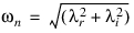
The model eigenvalues are reported to the workstation screen. In general, the eigenvalues are complex values, made up of real and imaginary components. The imaginary component represents the damped natural frequency  . The damping ratio must be less than 1 in order to produce an imaginary component in the eigenvalue - in other words, the damped natural frequency is zero whenever the damping ratio is 1 or greater.
. The damping ratio must be less than 1 in order to produce an imaginary component in the eigenvalue - in other words, the damped natural frequency is zero whenever the damping ratio is 1 or greater.The undamped natural frequency and damping ratio obeys the following equations:

where:
■ is the real part of eigenvalue.
is the real part of eigenvalue. ■ is the imaginary part of eigenvalues.
is the imaginary part of eigenvalues. ■ is the undamped natural frequency.
is the undamped natural frequency. ■ is the damping ratio (
 < 1).
< 1).
is the damping ratio (< 1). The relationship between the damped natural frequency,  , and undamped natural frequency,
  , is:
, is:
, and undamped natural frequency, , is: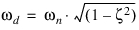
The damped natural frequency is the actual frequency at which the system is oscillating for that mode.
5.1.2 Using the RM option
By default (if no RM option and no PSTATE option are used), Adams Solver (C++) uses the global displacements and global rotations about the ground origin of all PARTS to build the linearized equations of motion. The complete set of defaults coordinates is shown in the next table.
Default linearization coordinates (no RM, no PSTATE options used) |
|---|
■Global displacements of the BCS of all PARTS, FLEX_BODY and POINT_MASS relative to the ground coordinate system, namely DX(BCS), DY(BCS) and DZ(BCS). |
■Global rotations of the BCS of all PARTS and FLEX_BODY relative to the ground coordinate system, namely AX(BCS), AY(BCS) and AZ(BCS). |
■All active modal coordinates in FLEX_BODY. |
■Global position, rotational vector, and slope of each node of FE_Part relative to the ground coordinate system |
■All states in LSE, TFSISO, LSE and GSE objects. |
■All states in DIFF objects. |
Note: | BCS stands for an internal MARKER located at the Body Coordinate System which is the location specified by the QG and REULER arguments of the PART, FLEX_BODY and POINT_MASS statements. |
The default linearization coordinates are not a minimal set. Therefore, Adams Solver (C++) selects an optimal subset x (the state variables) and linearizes the system in terms of those variables. As mentioned above, the default coordinate selection may not be the best choice in cases of rotating or accelerating systems. The first tool to customize the state variables is the RM option. The RM option sets the ADAMS id of a MARKER, for example:
LINEAR/EIGENSOL, RM=b
MARKER/b may be located on a rotating hub or accelerating subsystem of the model. When the option RM is used, the default coordinates are the following:
Default linearization coordinates using RM=b |
|---|
■Relative displacements of the BCS of all PARTS, FLEX_BODY and POINT_MASS relative to MARKER/b, namely DX(BCS,b,b), DY(BCS,b,b) and DZ(BCS,b,b). There is one exception: for the PART that owns MARKER/b, the default coordinates are DX(GROUND,b,b), DY(GROUND,b,b) and DZ(GROUND,b,b). |
■Relative rotations of the BCS of all PARTS and FLEX_BODY relative to MARKER/b, namely AX(BCS,b), DY(BCS,b) and DZ(BCS,b). There is one exception: for the PART that owns MARKER/b, the default coordinates are AX(GROUND,b), AY(GROUND,b) and AZ(GROUND,b). |
■All active modal coordinates in FLEX_BODY. |
■RM has no influence for FE_Part in selecting its linearization states. |
■All states in LSE, TFSISO, LSE and GSE objects. |
■All states in DIFF objects. |
The RM option is useful in linearizing helicopter blades, turbines, etc. If no RM option is used, the computed frequencies reflect a dependency on the rotation frequency, hiding the frequencies of interest. When the RM option is used, Adams Solver (C++) selects a subset x of the coordinates shown in the table above to perform the linearization.
Figure 6 Rotating spring-mass system
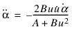
The exact equations of motion in terms of the shown coordinates are the following:
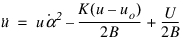
where:

Setting m1=m2=3, I1=I2=10, e=1, K=5, uo=10 and selecting an operating point defined by t=0, α =10, u=0,  =0,
=0,  =0, we obtain that one eigenvalue is zero and the other is 2.63056 Hz.
=0, =0, we obtain that one eigenvalue is zero and the other is 2.63056 Hz.The corresponding Adams dataset file is:
UNITS/FORCE = NEWTON, MASS = KILOGRAM, LENGTH = METER, TIME = SECOND
PART/1, GROUND
MARKER/6, PART = 1
PART/2, MASS = 3, CM = 7, IP = 10, 10, 10, WZ = 10
MARKER/5, PART = 2
MARKER/7, PART = 2, QP = 1, 0, 0
MARKER/10, PART = 2, REULER = 90D, 90D, 0D
PART/3, MASS = 3, CM = 8, IP = 10, 10, 10, WZ = 10
MARKER/8, PART = 3, QP = 10, 0, 0
MARKER/9, PART = 3, REULER = 90D, 90D, 0D
JOINT/1, REVOLUTE, I = 5, J = 6
JOINT/2, TRANSLATIONAL, I = 9, J = 10
SPRINGDAMPER/1, TRANSLATIONAL, I = 6, J = 8, K = 5, L = 10
ACCGRAV/I=0, J=0, K=0
RESULTS/XRF
END
PART/2 corresponds to the first link and PART/3 is the mass on the tip. Computing an eigensolution using the default command LINEAR/EIG, we obtain the following results shown in the message file:
This model has
4 kinematic states (displacement and velocities)
0 differential states (DIFFs, LSEs, etc.)
The selected kinematic states are:
1 Global rotation AZ(BCS) PART/2
2 Global displacement DX(BCS) PART/3
The other kinematic states are the respective derivatives.
E I G E N V A L U E S at time = 0.00000E
Number Real(cycles/unit time) Imag.(cycles/unit time)
1 0.00000E
2 0.00000E
3 0.00000E 3.07455E
Notice that the selected states are the global rotation of PART/2 about the z-axis (AZ(BCS) PART/2) and the global x-displacement of PART/3 (DX(BCS) PART/3). While the first one coincides with the coordinate alpha used to generate the equations of motion, the second one does not correspond to coordinate u.
The correct results are obtained using the following command:
LINEAR/EIGEN, RM=5
Where MARKER/5 is located on the first link. The corresponding results are:
This model has
4 kinematic states (displacement and velocities)
0 differential states ( DIFFs, LSEs, etc.)
The selected kinematic states are:
1 Relative rotation AZ(GROUND,5) PART/2
2 Relative displacement DX(BCS,5,5) PART/3
The other kinematic states are the respective derivatives.
E I G E N V A L U E S at time = 0.00000E
Number Real(cycles/unit time) Imag.(cycles/unit time)
1 0.00000E
2 0.00000E
3 0.00000E 2.63056E
Notice that the selected states now coincide with α and u and that the results match the theoretical ones.
For an example of using RM, see Simcompanion Knowledge Base Article KB8016438.
5.1.3 Using the PSTATE option
The PSTATE option is used to indicate the ADAMS ID of a PSTATE object. A PSTATE object is a set of VARIABLES defining user-defined coordinates (see the PSTATE statement). You may want to linearize the system using specific coordinates that the RM option does not provide. The methodology is:
1. Create as many variables as user-defined coordinates you want Adams Solver (C++) to use when linearizing the model.
2. Create a PSTATE object and enter the Adams id of all variables created in the previous step.
3. Issue a LINEAR/EIGEN command using the PSTATE=id option.
The following example illustrates these steps.
Figure 7 Simple model of a rigid helicopter blade
Figure 7 shows a simplified model of a rigid helicopter blade where the first link has a prescribed angular velocity w. Observe that the system has one degree of freedom but there are several coordinates to choose from to build the equations of motion. The classical approach is to use angle  but there may be a requirement to use coordinate y instead.
but there may be a requirement to use coordinate y instead.If the angle  is used, the equation of motion is:
is used, the equation of motion is:
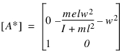
Linearizing this equation in terms of  the following state matrix is obtained (at time t=0):
the following state matrix is obtained (at time t=0):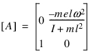
and the corresponding frequency is
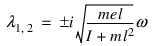
where i is the imaginary constant. Setting m=3, e=2, l=10, I=10, and w=10, we obtain  = 0.70019 Hz.
= 0.70019 Hz.The corresponding Adams dataset is:
UNITS/FORCE=NEWTON, MASS=KILOGRAM, LENGTH=METER, TIME=SECOND
PART/1, GROUND
MARKER/6, PART = 1
PART/2
MARKER/5, PART = 2
MARKER/8, PART = 2, QP = 2, 0, 0
PART/3, MASS = 3, CM = 10, IP = 0, 0, 10, WZ = 10
MARKER/7, PART = 3, QP = 2, 0, 0
MARKER/10, PART = 3, QP = 12, 0, 0
MARKER/12, PART = 3, QP = 22, 0, 0
JOINT/1, REVOLUTE, I = 5, J = 6
JOINT/2, REVOLUTE, I = 7, J = 8
MOTION/1, ROTATIONAL, JOINT = 1, FUNCTION = 10*TIME
ACCGRAV/I=0, J=0, K=0
RESULTS/XRF
END
where PART/2 is the first link and PART/3 is the rigid blade. Running the model with a LINEAR/EIG command, we obtain the following output:
This model has
2 kinematic states (displacement and velocities)
0 differential states ( DIFFs, LSEs, etc.)
The selected kinematic states are:
1 Global rotation AZ(BCS) PART/3
The other kinematic states are the respective derivatives.
E I G E N V A L U E S at time = 0.00000E
Number Real(cycles/unit time) Imag.(cycles/unit time)
1 0.00000E 7.00188E-01
Notice the exact match with the theoretical results. However, let's assume you want to linearize the model using coordinate y instead. If that is the case, the state matrix is now:
and the frequencies are:
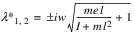
Using the same physical parameters, the frequency turns out to be  = 1.73867 Hz. To obtain this second result, add the following lines to the dataset file:
= 1.73867 Hz. To obtain this second result, add the following lines to the dataset file:VARIABLE/1, FUN=DY(10)
PSTATE/1, VAR=1
Notice that MARKER/10 is located on the CM of the blade, therefore DY(10) is the coordinate y shown in the figure above. Re-running the model using the following command:
LIN/EIGEN, PSTATE=1
The corresponding results are:
This model has
2 kinematic states (displacement and velocities)
0 differential states (DIFFs, LSEs, etc.)
The selected kinematic states are:
1 PSTATE VARIABLE VAR/1 DY(10)
The other kinematic states are the respective derivatives.
E I G E N V A L U E S at time = 0.00000E
Number Real(cycles/unit time) Imag.(cycles/unit time)
1 0.00000E 1.73876E
Notice that the results match the theory.
The documentation for the PSTATE statement provides guidelines for the correct definition of user-defined coordinates. Below is a brief summary:
■The VARIABLE's function expression must define a non constant displacement or angular measure.
■The displacement or angular measure can be global or relative.
■The number of user-defined coordinates can be less than the number of degrees of freedom of the model. Adams Solver (C++) will complete the state array using coordinates taken from the set of default coordinates.
■The number of user-defined coordinates can be greater than the number of degrees of freedom of the model. Adams Solver (C++) selects the required number, ignoring the rest.
■Redundant definitions will be rejected.
■Adams Solver (C++) may ignore a user-defined coordinate if there is already an equivalent default definition.
For an example of using PSTATE, see Simcompanion Knowledge Base Article KB8016414
5.1.4 Using both the RM and PSTATE options
You may safely use both the RM and the PSTATE options. Adams Solver (C++) assigns a higher priority to the user-defined states specified by the VARIABLES referenced in the PSTATE object. Default coordinates generated by the RM option have a lower priority.
Note: | RM option has no influence for FE_Part in selecting its linearization states. FE_Part will always use global position, rotational vector, and slope of each node relative to the ground coordinate system as its linearization states. |
For example, the following command linearizes the model using both options.
LINEAR/EIGEN, RM=77, PSTATE=3
5.1.5 Coordinates, Kinetic, Dissipative and Strain options
If you specify the COORDS, KINETIC, DISSIPAT, STRAIN, FCOORDS, FKINETIC, FDISSIPAT or FSTRAIN arguments, Adams Solver (C++) computes tabular output tables and writes them to an ASCII text file. The name of the text file has the same base name as the message file and it has an extension *.txt. For each mode in the specified mode range or frequency range, the printed output could consist of up to five sections.
The first section is a header that contains the mode number, undamped natural frequency, the absolute value of the damping ratio, generalized stiffness, generalized mass and model energy for the mode. Generalized stiffness and generalized mass are in user-specified units. See section Units in Coordinates, Kinetic, Dissipative and Strain modal tables for units used in the tables.
The following lines show the eigenvalues of simple model (this output is taken from a message file). In this particular case all eigenvalues have an imaginary part:
E I G E N V A L U E S at time = 0.00000E+00
Number Real(cycles/unit time) Imag.(cycles/unit time)
1 0.00000E+00 +/- 1.59155E+01
2 0.00000E+00 +/- 2.75664E+01
Assuming the above eigensolution was generated using the command:
linear/eigen, coords=1,2, kinetic=1,2, dissipat=1,2, strain=1,2
The corresponding tabular output found in the text file for mode number 1 looks as follows:
------------------------------------------------------------------
Energy table for MODE 1
------------------------------------------------------------------
Damping ratio = 1.20792E-15
Undamped natural freq. = 1.59155E+1 Cycles per unit time
Generalized stiffness = 2.00000E+0 User mass/time^2
Generalized mass = 2.00000E-4 User mass
Kinetic energy = 1.00000E+0 User mass/time^2
For the case of a vibrational mode, Adams Solver (C++) defines the following quantities:
e = a + bi
damping ratio = abs(a / undamped natural freq.)
Undamped natural freg. = 
Where e=a+bi is the corresponding eigenvalue. In case the magnitude of the eigenvalue is zero, the damping ratio is defined as zero. Notice above the printed value of the first eigenvalue's real part is zero. However, this is just a formatting choice to print zeros for very small numbers. The real part is very small hence the small value for the damping ratio printed in the header above.
The following lines show the eigenvalues of second simple model where all eigenvalues don't have imaginary parts:
E I G E N V A L U E S at time = 0.00000E+00
Number Real(cycles/unit time) Imag.(cycles/unit time)
1 -6.83125E-01
2 -2.24739E+00
3 -1.47243E+04
4 -7.57688E+05
This corresponding header for the first mode is now:
------------------------------------------------------------------
Energy table for MODE 1
------------------------------------------------------------------
Damping ratio = 1.00000E+0
Undamped natural freq. = 6.83125E-1 Cycles per unit time
Generalized stiffness = 4.08401E+1 User mass/time^2
Generalized mass = 2.21680E+0 User mass
Kinetic energy = 2.04201E+1 User mass/time^2
For the case of non-vibrational modes (imaginary part is zero), the damping ratio and undamped natural frequencies are defined by Adams Solver (C++) as:
e = a + 0 * i
damping ratio = 1.0
Undamped natural freg. = abs(a)
In all cases (for either real-only or imaginary eigenvalues), the generalized stiffness, generalized mass and kinetic energy are defined as follows:
Generalized mass = 2 * (Total energy)
Kinetic energy = 2.0 * (Generalized mass) * (undamped freq)2 * 
Generalized stiffness = 2 * (Kinetic energy)
Where a is real part of the corresponding eigenvalue. The Total energy is computed as the summation of all the kinetic energy corresponding to all rigid and flexible inertial objects in the Adams model. The kinetic energy is computed with the velocity entries in the corresponding eigenvector. See more details on the kinetic energy computation in Section 5.1.6.
The second section is a table of coordinates if the COORDS or FCOORDS argument is specified. This section is not output if the COORDS or FCOORDS argument is not specified or if the particular mode number is not within the range specified on the COORDS or FCOORDS argument. Each part in the Adams Solver (C++) model has one row in this table. The part translational coordinates in columns labeled (X,Y, and Z), represent the small translational displacements of the part center-of-mass (cm) marker in the global reference frame. The part rotational coordinates, in columns labeled (RX, RY, and RZ), represent the small rotational displacements of the part about the global x, y and z axes, respectively. Each coordinate in this table is represented by a magnitude and a phase. The mode is normalized so that the largest component in the mode has a value of 1.0 and a phase angle of 0 degrees. Magnitude and phase of all other components in the mode are reported relative to this largest component. Phase angles are represented in the range 0 to 355 degrees. Phase angles in the range 175 to 185 degrees are reported as 180 degrees. Phase angles in the range 355 to 360 degrees as well as phase angles in the range zero to five degrees are reported as zero degrees. States of elements resulting in user supplied differential equations are also represented in the coordinate table. All components with zero magnitude are also reported as having zero phase angles.
The third section is a table of modal kinetic energy distribution if the KINETIC or FKINETIC arguments are specified. This section is not present in the output for a particular mode if the mode number is not within the range of the modes specified on the KINETIC or FKINETIC arguments. Each part is represented by a single row in this table. Each entry in this table represents the percentage of the total modal kinetic energy for that part in a particular direction. Translational directions in which the modal kinetic energy distribution is computed are x, y and z displacement of the part center-of-mass (cm) in the global reference frame. Rotational directions are denoted by RXX, RYY, and RZZ; these represent the small displacement rotations of the part about the global x, y and z axes, respectively. The cross rotations are represented as RXY, RYZ, and RXZ. The sum of all values in a modal energy distribution table should be 100.0. Elements resulting in user-supplied differential equations are not considered in the computation for this table.
The fourth section is a table of modal strain energy distribution if the STRAIN or FSTRAIN argument is specified. This section is not present in the output for a particular mode if the mode number is not within the range of the modes specified on the STRAIN or FSTRAIN argument. Each force element is represented by one or more rows in this table. The table below shows the contribution of various element types to this table. Computation of strain energy accounts for the direct and indirect dependence of the force on PART displacements. The indirect dependence on PART displacements may be through dependence of the force on other FORCEs, VARIABLEs, or algebraic DIFFs that may be directly or indirectly dependent on PART displacements.
Elements Contributing to Table for Dissipative and Strain Energy Computations
Total | X | Y | Z | RX | RY | RZ | |
|---|---|---|---|---|---|---|---|
BEAM | X | X | X | X | X | X | X |
BUSHING | X | X | X | X | X | X | X |
CONTACT | X | X | X | X | X | X | X |
FIELD | X | X | X | X | X | X | X |
GFORCE | X | X | X | X | X | X | X |
NFORCE for marker 1 | X | X | X | X | X | X | X |
... | X | X | X | X | X | X | X |
for marker n | X | X | X | X | X | X | X |
SFORCE (translational) | X | X | X | X | |||
SFORCE (rotational) | X | ||||||
SPRINGDAMPER (translational) | X | X | X | X | |||
SPRINGDAMPER (rotational) | X | ||||||
VFORCE | X | X | X | X | |||
VTORQUE | X | X | X | X |
In the table, X, Y, and Z refer to translation components along the global x, y and z directions and RX, RY, and RZ refer to rotational components about the global x, y and z directions. An X indicates locations for contributions for individual elements. The column labeled Total contains a summation of the strain/dissipative power contribution due to the element in various directions.
The fifth section is a table of modal dissipative power distribution if the DISSIPAT or FDISSIPAT argument is specified. This section is not present in the output for a particular mode if the mode number is not within the range of the modes specified on the DISSIPAT or FDISSIPAT argument. Each force element is represented by one or more rows in this table. The table shows the contribution of elements to this table. Computation of dissipative power accounts for the direct and indirect dependence of the force on PART velocities. The indirect dependence on PART velocities may be through dependence of the force on other FORCEs, VARIABLEs, or algebraic DIFFs that may be directly or indirectly dependent on PART velocities.
By default, all tabular real data is printed using a format displaying only two decimal values. If engineering format is required, use the TABLE_PRECISION option with a value bigger than 2. If the precision is set to 3 or bigger, an engineering (exponential) format is use. Moreover, option NAMES will force Adams Solver (C++) to add the Adams View names found in the Adams modeling database.
5.1.6 Further details on kinetic energy tables
Modal energy tables are printed to an ASCII *.txt file when the options KINETIC or FKINETIC are used. This section provides more details on how the kinetic energy tables are computed for the case of rigid PARTs and FLEX_BODIES. The case of POINT_MASSs is handled similarly. Figure 8 (a) shows a typical PART at the moment a linearization command is issued. Notice the principal inertia frame 1-2-3 of this PART (in blue color) is not necessarily coincident with the global reference frame x-y-z shown in black. At the current principal orientation 1-2-3 the inertia tensor I (considering only the rotational coordinates) is the following:
The first step in preparing the contribution of this PART to the kinetic energy tables is to transform the principal inertia tensor expressing it in global coordinates coincident with the x-y-z frame as shown in Figure 8 (b).
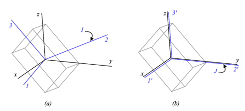
Figure 8 A PART at the current linearization state.
The inertia tensor of this PART expressed in global coordinates x-y-z is the following:
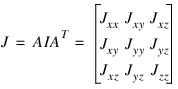 .
.Where A is the local kinematic transformation from the 1-2-3 frame to the global frame. Notice the terms  ,
,  and
and  can be negative. With the inertia tensor aligned with the global reference frame, the kinetic energy K has this expression:
, and can be negative. With the inertia tensor aligned with the global reference frame, the kinetic energy K has this expression: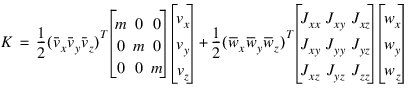
In the above expression, a variable  with an overbar represents the complex conjugate of z. In order to compute the kinetic energy, velocities and angular velocities are extracted from the corresponding mode shape. In general, these quantities are complex numbers. However, given the symmetry of the inertia tensors, it can be demonstrated that the above expression for the kinetic energy is always a real number bigger or equal than zero. Introducing the following terms:
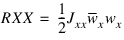
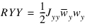
with an overbar represents the complex conjugate of z. In order to compute the kinetic energy, velocities and angular velocities are extracted from the corresponding mode shape. In general, these quantities are complex numbers. However, given the symmetry of the inertia tensors, it can be demonstrated that the above expression for the kinetic energy is always a real number bigger or equal than zero. Introducing the following terms: ,
,

 .
.the kinetic energy K can be rewritten as:
 .
.Notice that the terms associated with cross products (RXY, RXZ and RYZ) can be negative when the transformation of the principal moment of inertia from local to global coordinates results in negative products of inertia (off-diagonal terms).
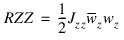
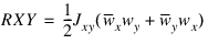
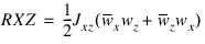
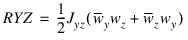
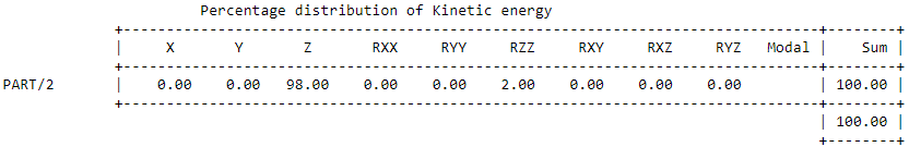
Adams Solver computes the quantities X, Y, Z, RXX, RYY, RZZ, RXY, RXZ and RYZ and prints them as shown below.
The kinetic energy for FLEX_BODYs has the following expression:
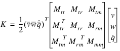 .
.Here v, w and  stand for vector quantities (velocity, angular velocity and modal velocities respectively) and the overbar indicates a complex conjugate. The notation matches that of the FLEX_BODY theoretical documentation.
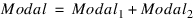
stand for vector quantities (velocity, angular velocity and modal velocities respectively) and the overbar indicates a complex conjugate. The notation matches that of the FLEX_BODY theoretical documentation.Notice matrix Mtt is a 3x3 diagonal matrix with the total mass of the body in the diagonal terms. Notice also that matrix Mrr is similar to the inertia tensor of a rigid PART. Hence, the contributions of the rigid body motion of the FLEX_BODY is computed exactly the same way as computed for a rigid PART. Therefore the kinetic energy of a FLEX_BODY is expressed as:

Where Modal has the following expression:
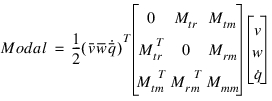
Previous to version Adams 2013, the Modal contribution was not reported; that was the reason the kinetic energy did not sum up to 100% in models having flexible bodies.
Starting Adams 2013, the energy tables do report the Modal values along with the total kinetic energy per body. An example typical table is shown below.
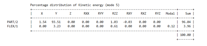
Notice in this example the RXY contribution of the rigid PART/2 is negative. Notice also the Modal contribution is particularly important in this case.
5.1.7 Kinetic energy reported in Adams View
Previous section describes the ASCII *.txt output generated by Adams Solver in batch mode or when running the external solver from Adams View. When running the internal solver, the Modal kinetic energy reported by Adams View is split into two terms. The Modal contribution is rewritten as follows:
Where

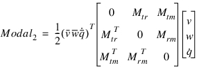
Term Modal1 is displayed in a two-column table showing the contribution of each individual mode i and corresponding value  . Term Modal2 is lumped into a single number called Offset Diagonal Coupling.
. Term Modal2 is lumped into a single number called Offset Diagonal Coupling.5.1.8 Modal Energies Computed by Solver
For a general linear system of equations:
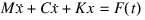
 ,
, 
where  is the generalized coordinates (S_variables),
  is the modal coordinates (natural coordinates),
  is displacement modal matrix and
  is the displacement mode shape vector i. and
  and
and  are square matrices with dimensions similar to S_variables vector dimension.
is the generalized coordinates (S_variables), is the modal coordinates (natural coordinates), is displacement modal matrix and is the displacement mode shape vector i. and and are square matrices with dimensions similar to S_variables vector dimension.Now define
And furthermore,
 ,
,  and
and 
The modal coordinates and modal velocities are obtained from
 and
and 
And the modal mass, stiffness and damping matrices are obtained from,
 ,
,  and
and 
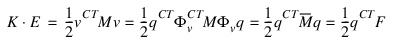
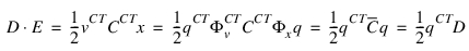
The kinetic energy is defined as,
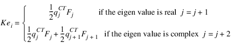
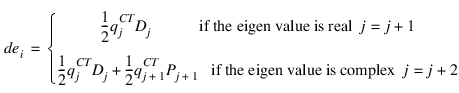
The kinetic energy per mode i is computed as,
The potential energy is defined as,

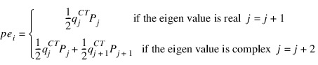
The potential energy per mode i is computed as,
The dissipative power is defined as,
The dissipative power per mode i is computed as,
Note that if the modal matrix,  is singular,
is singular, cannot be determined, modal energies cannot be computed and Adams solver will issue an error.
5.1.9 Modal Effective Mass and Participation Factors Computed by Solver
The vector of modal participation factor is defined as,
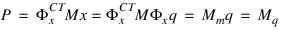
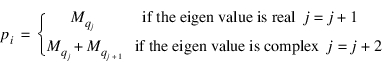
The modal participation factor for mode i is defined as,
The vector of modal participation factor is defined as,

Then the effective mass per mode is calculated as,
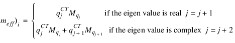
Here, the superscript C stands for the complex conjugate
5.1.10 Differences in results compared with Adams Solver FORTRAN
Adams Solver FORTRAN uses an old linearization technology limited to providing good results for static cases only. Adams Solver FORTRAN finds the linearization matrix by assembling the static equations and extracting the linearization matrix from the statics equations to solve. Perhaps the major limitation of Adams Solver FORTRAN is that the linearization matrix is obtained in terms of the simulation states only (global translations and global Euler angles). Adams Solver C++, on the other hand, uses a modern and general algorithm suitable for all operating points (static and dynamic) with no simplifications. Moreover, Adams Solver C++ can linearize the system in terms of arbitrary coordinates; its algorithm is not constrained to use the coordinates used in formulating the equations of motion, any coordinate definition can be chosen. Users may also define the linearization states to be used in the linearization and obtain custom linear representations for the system.
Regardless of the implemented linearization algorithm, the first step is the selection of the independent states for the linearization. The independent states correspond to the minimal state-space representation of the system. When using Adams Solver FORTRAN, the independent states are a subset of the coordinates used to solve the equations of motion (global translations, global Euler angles, differential states). When using the Adams Solver C++, the default linearization states are a subset of global translations and instantaneous global rotations about GROUND origin. The decision was made based on the popularity of global rotations in FEA codes. Hence, the main difference between Adams Solver FORTRAN and Adams Solver C++ is the set of linearization states. Although linearization states may be different, eigenvalues may match (see reference mentioned in Section 1.0). However, modal table results may be different but both are correct. To illustrate this point the model in Figure 9 shows a simple model of a vertical pendulum (red box with a hinge on top) connected by a spring-damper to GROUND (blue box on the right).
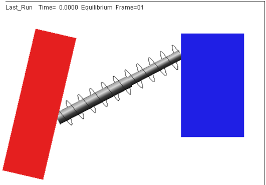
Figure 9 A simple pendulum with a spring-damper force.
The data set describing this model is presented in the Appendix, Listing 6, Listing 7 and Listing 8 show the command files *.acf used to linearize this model using Adams Solver FORTRAN and Adams Solver C++ respectively. Running both solvers the reader can verify both solvers provide the same eigensolution but different results in selected linearization states and different results in modal tables (generalized mass, general stiffness). Observing the message files created by both solvers we first notice the following. The FORTRAN solver reports:
SCRCRD:COORDS
Coordinate X of PART/2 (model_1.PART_2)
While the C++ solver reports:
The selected kinematic states are:
1 Global rotation AZ(BCS) PART/2
Notice the FORTRAN solver selected the horizontal displacement of PART/2 while the C++ solver selected the instantaneous rotation of PART/2 as the respective linearization states. Notice although different, the selected states provide the same eigenfrequency. However, inspecting the *.out file created by the FORTRAN solver, we find:
Damping ratio = 4.67704E-02
Undamped natural freq.= 9.59339E-01 Cycles per second
Generalized stiffness = 4.09672E+00 User mass/second^2
Generalized mass = 1.12754E-01 User mass
Kinetic energy = 2.04836E+00 User mass/second^2
While the results printed by the C++ solver (in an *.txt) file are:
Damping ratio = 4.67704E-2
Undamped natural freq. = 9.59339E-1 Cycles per unit time
Generalized stiffness = 1.74065E+5 User mass/time^2
Generalized mass = 4.79080E+3 User mass
Kinetic energy = 8.70325E+4 User mass/time^2
These results while different are correct given that the generalized mass and generalized stiffness are based on the mode shape which in turn depend on the selected linearization states. Nevertheless, the C++ solver can match the results of the FORTRAN solver by using the PSTATE option. In that regard, Listing 9 shows the command file used to run the C++ solver. Listing 9 executes the linearization using a custom coordinate defined by VARIABLE/5:
VARIABLE/5
, FUNCTION = DX(7)
VARIABLE/5 defines the global horizontal translation of PART/2 (used by the FORTRAN solver). Running the C++ solver and observing the message file we find:
The selected kinematic states are:
1 PSTATE VARIABLE VAR/5 DX(7)
This message means the C++ solver honored the request of the PSTATE option in the LINEAR command. The reader can now verify the *.txt created by the C++ solver matches the computation of the FORTRAN solver.
5.1.11 Advanced eigensolution issues
In case you need to compare the computed eigensolution with results from another software package, you may export the linearization matrices using the LINEAR/STATEMAT option. The exported [A] matrix is the one we send to the eigensolver.
In general, the issues affecting the quality of the eigensolution are the following:
a. Models in singular configurations. Models in singular configuration may report spurious modes and frequencies or they may report different values (with a sign reverse) under small perturbations.
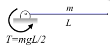
For instance, the beam shown in the figure above is at an unstable equilibrium position. A small perturbation moving the tip downward will cause the torque to restore the previous equilibrium position (complex eigenvalue). However, a small perturbation moving the tip upward will case the system to move away from the horizontal position (real eigenvalue). At exactly the horizontal position the eigenvalues are zero. Solving a complex system with the same overall topology may results in spurious eigenvalues.
b. Accelerating models. Accelerating or rotating components usually involve mode shapes involving velocity states and may show strange mode shapes.
c. Multiple rigid body modes. If the model has the potential to experiment rigid body motion, the eigensolver may show up with noisy frequencies instead of a zero value. This depends on the size of the model. Moreover, if the model has DIFFs or LSEs or GSEs or TFSISOs objects, then some modes will be related to the differential states with almost no coupling with overall motion of the system. Those modes will show no animation.
The issue of noisy frequencies when the model has rigid-body modes is a direct consequence of round-off errors in the linearization and round-off errors in the eigensolution algorithm. Users are encouraged to visually identify the rigid body modes using the mode animation tool.
The issue of noisy frequencies when the model has rigid-body modes is a direct consequence of round-off errors in the linearization and round-off errors in the eigensolution algorithm. Users are encouraged to visually identify the rigid body modes using the mode animation tool.
d. Overdamped models. Damping may create spurious modes that create clutter and make difficult to find the modes of interest. Since the damping is hard to estimate, we recommend also running the eigensolution with the NODAMP option to gain perspective on the interesting modes. Damping can be added afterward to estimate its influence in the solution.
e. Friction in stiction regime. If the model has FRICTION objects running in the stiction mode, you may get spurious frequencies and mode shapes due to the stiffness of the force element added to model the stiction.
f. Numerical limitations. In general, the linearization matrix [A] is non-symmetric, ill-conditioned and sparse. In addition, there is a natural limitation in the precision of the arithmetic operations of the computer. The end results may be that frequencies and mode shapes may include noisy results especially in both the lower end of the real eigenvalues (real-only eigenvalues with small values) and in the lower imaginary spectrum (complex eigenvalues with small imaginary part). Higher real-only eigenvalues and higher imaginary eigenvalues are usually better extracted.
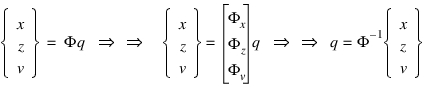
5.1.10 Eigenvectors and mode shapes
The technical literature usually makes no difference between an eigenvector and a mode shape by using the terms interchangeably. In Adams, however, we use the term eigenvector for the vectors z in the solution of the complex eigenproblem:

where matrix A corresponds to the minimum state-space representation of the model. The size of array z, in the most general case, has this value:
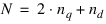
where  is the number of degrees of freedom and
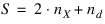
  is the number of differential equations in the model. The number of degrees of freedom is computed from:
is the number of degrees of freedom and is the number of differential equations in the model. The number of degrees of freedom is computed from:
where  is the number of coordinates used to define the model and m is the number of constraint equations. Adams Solver C++ does not scale the eigenvectors z nor makes them available for the user. If there is a need to obtain the z eigenvectors, the user may obtain the A matrix using the STATEMAT option and compute the eigenvectors using a third party code. Notice that
  which implies only a subset of all coordinates is used perform the linearization. Moreover, the user may define linearization states using the PSTATE option. In any case, the list of linearization states is printed in the message file and exported to a text file when using the STATEMAT option.
is the number of coordinates used to define the model and m is the number of constraint equations. Adams Solver C++ does not scale the eigenvectors z nor makes them available for the user. If there is a need to obtain the z eigenvectors, the user may obtain the A matrix using the STATEMAT option and compute the eigenvectors using a third party code. Notice that which implies only a subset of all coordinates is used perform the linearization. Moreover, the user may define linearization states using the PSTATE option. In any case, the list of linearization states is printed in the message file and exported to a text file when using the STATEMAT option.When using the Post-processor, the raw eigenvectors z are not usable for visualizing the vibrations of the model. In order to visualize the vibrations of the model, Adams defines the mode shapes as follows:

where matrix T is a transformation from the minimal state-space representation to the full set of coordinates used in the model. Matrix T is obtained during the reduction from the full Lagrange equations of motion to the minimum state-space representation. Mode shapes  are scaled by searching for the entry with the largest modulus and dividing the vector by the entry with the largest modulus.
are scaled by searching for the entry with the largest modulus and dividing the vector by the entry with the largest modulus. The size of the mode shapes is given by the following expression:
Mode shapes  are available to the user in the results files and they are used by the Post-processor to perform animations of the vibrating model. Mode shapes are also printed to a text file when using the COORD option in the LINEAR command.
are available to the user in the results files and they are used by the Post-processor to perform animations of the vibrating model. Mode shapes are also printed to a text file when using the COORD option in the LINEAR command.5.1.11 Units in Coordinates, Kinetic, Dissipative and Strain modal tables
Given that Modal coordinates tables, as well as kinetic, dissipative and strain energy tables are computed using normalized eigenvectors, length units have been dropped out.
For example, the generalized stiffness and the kinetic energy are displayed using units of User-mass/time^2:
-----------------------------------------------------------
Energy table for MODE 1
-----------------------------------------------------------
Damping ratio = 1.00000E+0
Undamped natural freq. = 6.83125E-1 Cycles per unit time
Generalized stiffness = 4.08401E+1 User mass/time^2
Generalized mass = 2.21680E+0 User mass
Kinetic energy = 2.04201E+1 User mass/time^2
Theoretically, energy has units of mass times velocity square. Dropping the length dimension, we obtain mass/time^2.
5.1.12 Option ORIGINAL
There are three important differences between the Adams Solver C++ and Adams Solver FORTRAN regarding the linearization implementation. Nevertheless, these differences can be controlled by the keyword ORIGINAL and/or three environment variables. The environment variables can be used independently in any combination.
a. As mentioned in section Differences in results compared with Adams Solver FORTRAN, for inertial elements (PARTs, FLEX_BODYs and so on) Adams Solver FORTRAN uses global positions and global Euler angles of the center of mass; Adams Solver C++, on the other hand, uses global positions and global instantaneous rotations by default.
To force Adams Solver C++, use the same coordinates used by Adams Solver FORTRAN, set the environment variable MSC_LINEAR_PBCS_STATES to any value.
b. When the model has differential states (DIFFs, GSEs, LSEs, TFSISOs), the linearization matrix has the following general form (see Normal Mode Analysis):
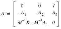
where submatrix A3 is the coupling between the differential states and the velocities. When using the NODAMP option, Adams Solver FORTRAN will flush the coupling terms (A3) while Adams Solver C++ will not flush the coupling terms. In other words, Adams Solver C++ does not consider the coupling terms to be some sort of damping.
To force Adams Solver C++ imitate Adams Solver FORTRAN into flushing the coupling terms, set the environment variable MSC_ADAMS_SOLVER_NODAMP_DIFF to any value.
To force Adams Solver C++ imitate Adams Solver FORTRAN into flushing the coupling terms, set the environment variable MSC_ADAMS_SOLVER_NODAMP_DIFF to any value.
c. Adams Solver FORTRAN will not reconcile the system before extracting the linearization matrix. As mentioned in section Differences in results compared with Adams Solver FORTRAN, Adams Solver FORTRAN re-uses the last Jacobian matrix to extract the linearization matrix. This behavior has some advantages when compared to the Adams Solver C++. Adams Solver C++ will reconcile the system (perform initial conditions analysis) to set the model in a consistent state if need be. Hence, linearization results can be different between the two solvers. For example, let's assume you have a model with DIFF statements using the STATIC_HOLD option. Let's assume you execute these commands:
simulate/static
linear/eigensol
Adams Solver FORTRAN will perform the linearization using the states computed from the previous static simulation; the differential states using STATIC_HOLD, are not modified during the static simulation. However, Adams Solver C++ considers the eigensolution a new simulation, hence it reconciles the system right before the linearization. This reconciliation will potentially modify the differential states used in the linearization, generating differences with respect to Adams Solver FORTRAN.
To force Adams Solver C++ not to reconcile before a linearization, set the environment variable MSC_ADAMS_LINEAR_NO_CHECKS_FOR_CONSISTENCY to any value.
Specifying option ORIGINAL is equivalent to setting the above three environment variables.
5.2 State matrices and MKB computation
5.2.1 Scope
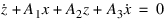
If you issue the LINEAR/STATEMAT command, Adams Solver (C++) computes the state matrices representation of the Adams model. The linearized Adams model is represented as:


where:
■Vector s represents the state variables of the plant model. The state variables can be user-defined coordinates (see the RM and PSTATE options). By default, the state variables are displacements, modal coordinates (from flexible elements) and their corresponding time derivatives. The state variables also include all of the differential states from DIFs, LSEs, GSEs and TFSISOs.
■Vector u represents the inputs of the plant model.
■Vector y represents the outputs from the plant model.
■Matrices A, B, C, and D are the state-space matrices representing the plant.
Matrices A, B, C and D are exported to the text file specified in the FILE option of the command. The exported text file includes a STATES matrix with information on the state vector s. Moreover, the export will create matrices PINPUT and POUTPUT with information on the inputs and outputs to the plant.
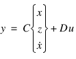
Vector s stands for the minimum state-space realization of the model. If you do not specify RM nor PSTATE options, Adams Solver (C++) will select the best choice of the coordinates in order to perform the linearization of the model. In general, vector s will have this format:
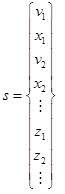
Where xi stands for a position state, vi stands for the corresponding time derivative, and zi stands for a differential state in the model. You could inspect vector s in the output file under the STATES matrix. See Section 5.2.6 for more information on the contents of the STATES matrix.
Caution: | Vector s has a different format if the MKB option is selected instead. |
By default all exported matrices (A, B, C, D, STATES, PINPUT, POUTPUT) are exported in a single file using the MATRIXX format. If you specify the FORMAT=MATLAB option in the command, then Adams Solver C++ will export up to seven files named xxxa, xxxb, xxxc, xxxd, xxxst, xxxpi and xxxpo, where 'xxx' stands for the root filename specified in the mandatory FILE=filename option of the LINEAR/STATEMAT command.
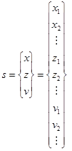
If you specify the MKB option, Adams Solver (C++) computes an alternative form of the state matrices representation for an Adams model. In this case, the linearized Adams model is first linearized in this format:
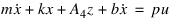
Where x are the position level linearization states and z stands for the differential states. Defining:

The state vector s is defined now as:
With this definitions the first equations of the state representation can be written as follows:
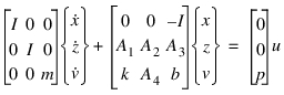
Defining:
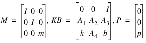
We obtain:
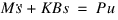

where:
■Vector s represents the state variables of the plant model. The state variables can be user-defined coordinates (see the RM and PSTATE options.) In this case the state variables are the displacements, modal coordinates (from flexible elements) and all differential states from DIFS, LSEs, GSEs and TFSISOs.
■Vector u represents the inputs of the plant model.
■Vector y represents the outputs from the plant model.
■Matrices M, KB, C, P and D are state matrices representing the plant.
Matrices M, KB, P, C and D are exported to the text file specified in the FILE option of the command. The exported text file includes a STATES matrix with information on the state vector s. Moreover, the export job will create matrices PINPUT and POUTPUT with information on the inputs and outputs to the plant.
The MKB option is useful if you need to export the Adams model to be a subsystem of an MSC.NASTRAN model.
5.2.2 Using the RM and PSTATE options
See sections Using the RM and PSTATE options.
5.2.3 Plant inputs and Plant outputs
You can specify the definition of plant inputs with the PINPUT argument value. Similarly, plant outputs are specified by the POUTPUT argument. States variables (x) are automatically selected by Adams Solver (C++) out of the total set of coordinates used to model the mechanical system. However, using the RM and/or the PSTATE options, you may have Adams Solver (C++) use user-defined coordinates for linearization. This is particularly important for rotating systems. While several PINPUT statements and POUTPUT statements may be present in an Adams model, you can specify only one of each on the LINEAR command.
Corresponding to each VARIABLE id specified on the PINPUT statement, a column exists in the B and D matrices (STATEMAT option). Similarly, for each VARIABLE id specified on the POUTPUT statement, a row exists in the C and D matrices. In effect, each VARIABLE id specified on the PINPUT or POUTPUT statement specifies an input or output channel, respectively.
Input channels are important in the computation of state matrices. It is important to notice that Adams Solver (C++) assumes the function expressions of all input channels are zero. If the function expression of an input VARIABLE is not zero, then you have two choices to properly model the system (assume the original input variable is VARIABLE/f):
1. Remove VARIABLE/f from the INPUT statement. This is usually the simples and correct choice.
2. Create a new VARIABLE/d and add it to the INPUT statement. Remove VARIABLE/f from the INPUT statement and modify its function expression to original_expression + VARVAL(d). Choose this approach if you need to keep the size of the B to an specified value.
Following the above recommendation you may properly model both open-loop and close-loop control systems.
Tip: | ■To reduce computing time, specify the NOVECTOR argument with the EIGENSOL option if mode shapes are not desired. ■Specify the LINEAR command to assess stability of Adams models by computing its eigenvalues. Eigenvalues with positive real parts correspond to unstable modes of the system. ■If you specify the PINPUT and the POUTPUT arguments for state matrices output, Adams Solver (C++) produces all four matrices (A, B, C, and D). If you do not specify the PINPUT argument, Adams Solver (C++) does not produce the B or D matrices. Similarly, if you do not specify the POUTPUT argument, Adams Solver (C++) will not produce the C or D matrices. If you do not specify either the PINPUT or POUTPUT arguments, Adams Solver (C++) produces only the A matrix. ■You may define several PINPUT and POUTPUT statements in an Adams Solver (C++) dataset, however, a LINEAR command allows only one PINPUT and one POUTPUT statement to be specified at a time. If you issue a series of LINEAR commands, Adams Solver (C++) computes alternate state matrix descriptions at the same operating point with different combinations of PINPUT and POUTPUT identifiers. Changes in the PINPUT and POUTPUT descriptions are reflected in the A, B, C, and D matrices. |
5.2.4 MATRIXX format
State matrices output by Adams Solver (C++) in the MATRIXX format conforms to the MATRIXx FSAVE ASCII file specification. These specifications are given in the Xmath Basics Guide, 1996, Integrated Systems Inc., Santa Clara, CA.
More than one matrix may be present in a single file. The Adams Solver (C++) state matrices file can have up to seven matrices. The first four matrices are the A, B, C, and D state matrices. The next three matrices are STATES, PINPUT, and POUTPUT. The contents and format of these matrices are explained in the next sections.
5.2.5 MATLAB format
State matrices output by Adams Solver (C++) in the MATLAB format conform to the ASCII flat file format. This format requires that all entries in a row of the matrix be written in a single record. Successive values in a row are separated by a single space. A file is allowed to contain only one matrix. Therefore, Adams Solver (C++) may create up to seven output files, one each for the A, B, C, and D matrices, one for STATES, one for PINPUT, and one for POUTPUT. The contents and format of the last three matrices are as shown in the next sections. The file name you specify is used as a base name and is appended with the matrix name to write the matrix of the appropriate type. The file names used for the seven matrices are as given in the table below.
File Names Used for MATLAB State Matrices Output
Matrix Name | file Name |
|---|---|
A | "base_name" "a" |
B | "base_name" "b" |
C | "base_name" "c" |
D | "base_name" "d" |
STATES | "base_name" "st" |
PINPUT | "base_name" "pi" |
POUTPUT | "base_name" "po" |
5.2.6 Contents of the STATES matrix
The STATES matrix contains information regarding states that Adams Solver (C++) has chosen for the state matrices representation. For each state, one record exists in this matrix. The following information is contained in each record:
Type_of_element | Element_identifier | Element_coordinate | Coordinate_value_at_operation_point |
Type_of_element
Type_of_element can take on the following values:
1. PART coordinates (using Euler angles)
2. States in a LSE element
3. States in a TFSISO element
4. States in a GSE element
5. Diff variable
6. Coordinate for a PTCV element
7. Coordinates for a CVCV element
8. FLEX_BODY element
9. POINT_MASS element
10. PSTATE variable (a VARIABLE used in a PSTATE object)
11. Derivative of a PSTATE variable
21. PART coordinates (no RM option was used)
27. FE_PART element
28. FLEX_BODY element (no RM option was used)
29. POINT_MASS element (no RM option was used)
31. PART coordinates (RM option was used)
38. FLEX_BODY element (RM option was used)
39. POINT_MASS element (RM option was used)
Element_identifier
Element_identifier is the eight-digit Adams Solver (C++) identifier of the element.
Element_coordinate
If Type_of_element=1, the Element_coordinate can take on the values:
1 Global x-displacement of PBCS (See the Note: below)
2 Global y-displacement of PBCS
3 Global z-displacement of PBCS
4 Global  angle of part principal axis of PBCS
angle of part principal axis of PBCS5 Global  angle of part principal axis of PBCS
angle of part principal axis of PBCS6 Global  angle of angle of part principal axis of PBCS
angle of angle of part principal axis of PBCS7 to 12 Correspond to the respective derivatives
Note: | PBCS stands for Principal Body Coordinate System. PBCS is a frame coincident with the PARTs CM MARKER but it is oriented along the principal inertia axis. PBCS is an internal MARKER used by Adams Solver (C++) to build the equations of motion. |
If Type_of_element=21, the Element_coordinate can take on the values:
1 Global x-displacement of BCS (See the Note: below)
2 Global y-displacement of BCS
3 Global z-displacement of BCS
4 Global rotation of BCS about the global x-axis
5 Global rotation of BCS about the global y-axis
6 Global rotation of BCS about the global z-axis
7 to 12 Correspond to the respective derivatives
Note: | BCS stands for Body Coordinate System. For details on BCS, see the PART command. |
If Type_of_element=31, the Element_coordinate can take on the values:
1 Relative x-displacement of BCS with respect to the RM marker
2 Relative y-displacement of BCS with respect to the RM marker
3 Relative z-displacement of BCS with respect to the RM marker
4 Relative rotation of BCS about the x-axis of the RM marker
5 Relative rotation of BCS about the y-axis of the RM marker
6 Relative rotation of BCS about the z-axis of the RM marker
7 to 12 Correspond to the respective derivatives
If Type_of_element=27, the Element_coordinate can take on the values depending on the DOF index in the FE_Part.
For Type_of_element=2 to 5, Element_coordinate is the sequence number in the set of states defining that element.
For Type_of_element=6, the only permissible value for Element_coordinate is 1, that is, the alpha parameter value that defines the contact point on the curve.
For Type_of_element=7, Element_coordinate may take on the value of 1 or 2, representing the parameter values for the first (I) or second (J) curve in a CVCV statement that defines the contact point on the curve.
For Type_of_Element=8, the Element_coordinate can take on the values:
1 - 12 same as for Type_of_Element=1
1 E6 + n nth modal generalized coordinate
2 E6 + n first time derivative of the nth modal generalized coordinate
1 E6 + n nth modal generalized coordinate
2 E6 + n first time derivative of the nth modal generalized coordinate
For Type_of_Element=28, the Element_coordinate can take on the values:
1 - 12 same as for Type_of_Element=21
1 E6 + n nth modal generalized coordinate
2 E6 + n first time derivative of the nth modal generalized coordinate
For Type_of_Element=38, the Element_coordinate can take on the values:
1 - 12 same as for Type_of_Element=31
1 E6 + n nth modal generalized coordinate
2 E6 + n first time derivative of the nth modal generalized coordinate
For Type_of_Element=9, the Element_coordinate can take on the following values:
1 - 3 same as for Type_of_Element=1
4 - 6 Correspond to the respective derivatives
4 - 6 Correspond to the respective derivatives
For Type_of_Element=29, the Element_coordinate can take on the following values:
1 - 3 same as for Type_of_Element=21
4 -6 Correspond to the respective derivatives
For Type_of_Element=39, the Element_coordinate can take on the following values:
1 - 3 same as for Type_of_Element=31
4 -6 Correspond to the respective derivatives
For Type_of_Element=10, the Element_coordinate takes the value 1.
For Type_of_Element=11, the Element_coordinate takes the value 2.
In the MATRIXX format, this data is organized in column order form so that the STATES matrix contains three rows and number of columns is equal to the number of states in the model. In the MATLAB format, this data is organized in the row order form. Therefore, the STATES file contains data organized in the three columns and the number of rows is equal to the number of states in the model.
For example, find the states used by the linearization computation from the listing shown below (the listing is obtained by using the FILE and MATRIXX options in a STATEMAT or MKB)
STATES 3 2 0(3(1PE25.17))
2.10000000000000000e+01 3.00000000000000000e+00 1.20000000000000000e+01
2.10000000000000000e+01 3.00000000000000000e+00 6.00000000000000000e+00
The first column shows a 21, which stands for a PART. No option RM was used in the linearization command. The second column shows a 3 which stands for the ADAMS id of the PART. The third column shows a 12 and a 6, therefore the states used by the linearization are:
1. Global rotation of the BCS of PART/3 about the global z-axis
2. The derivative of the global rotation of the BCS of PART/3 about the global z-axis.
5.2.7 Contents of the PINPUT and POUTPUT matrices
The first entry in the PINPUT (or POUTPUT) exported data contains the Adams Solver (C++) identifier of the PINPUT (or POUTPUT) statement that was used on the LINEAR command to generate the state matrices. Subsequent entries contain the Adams Solver (C++) identifiers of the VARIABLEs defining the PINPUT (or POUTPUT) statement. Using either the MATRIXX or the MATLAB format option, this data is organized as a matrix with 1 column and number of rows equal to one plus the number of variables on the PINPUT (or POUTPUT) statement.
All data for the STATES, PINPUT, and POUTPUT matrices is written as floating point data.
5.3 Nastran bulk data deck export
5.3.1 Scope
Using the EXPORT option Adams Solver (C++) exports the linearized Adams model as a set of Nastran bulk data deck files. The Nastran bulk data deck export is also known as "Adams-to-Nastran". In a few words, this option creates an equivalent Nastran model (linear model) equivalent to the Adams model at the operating point when the export command is executed. Adams-to-Nastran can be seen as a model translation process. The translation process is done with high fidelity. For medium to small models, eigenvalues computed in the Adams environment will match eigenvalues computed in the Nastran environment.
The syntax to invoke the EXPORT job calls for the type of export (OPENBOX or CLOSEDBOX), the name of the main bulk data deck file to be created (FILE argument), and an optional name for a configuration file (CONFIG argument). The configuration file is useful to customize the export process.
The translation process supports two types of EXPORT jobs, namely, a OPENBOX option or a CLOSEDBOX option which must be specified using the TYPE argument. These two types are conceptually different. Using the CLOSEDBOX option, Adams Solver (C++) computes the MKB matrices and exports the model as a set of three DMIGs. Individual contributions to the MKB matrices from all of the inertial elements, applied forces and constraints cannot be identified, hence the exported model is practically non modifiable. On the other hand, using the OPENBOX option, the linearized model is exported as a set of Nastran cards where an element-to-element translation takes place; this option exports a model that can be further edited and modified.
Using the EXPORT option, a configuration file can be specified to fine tune the export job. The syntax of the configuration file allows the user to select the solution number, specify exported MARKERS, single out applied forces, change the default numbering of GRID and other Nastran cards, select include directories, choose a type of graphical output, select a style of file generation, etc.
5.3.2 Limitations
There are no limitations on the type of previous analysis prior to the invocation of the LINEAR/EXPORT command if using the CLOSEDBOX export type. Also, eigenvalues computed by Nastran on the exported model will match eigenvalues computed by Adams on the Adams model. In a few words, both, static and dynamic operating points are supported by the CLOSEDBOX export.
When using the OPENBOX export type, we guarantee matching eigenvalues computed by both, Nastran and Adams, only if the operating point is a static one (if the previous simulation in Adams was either STATIC or QUASISATIC). Notice that a STATIC simulation at time t=0 may not be a truly static operating point because Adams Solver restores the initial velocities found in the model. This restoration of velocities after a STATIC simulation at time t=0 can be avoided by setting the environment variable MSC_ADAMS_STATICS_NO_RESTORE_VELOCITIES.
If the previous simulation done by Adams is a dynamic or kinematic analysis, the exported model includes TIC cards defining the velocities of the model. However, eigenvalues computed by both, Nastran and Adams will not necessarily match. This is not a limitation on the Adams side but a limitation inherent to most linear/nonlinear Finite Element codes available in the market.
If the operating point is KINEMATIC (no degrees of freedom), the only type allowed is OPENBOX. No CLOSEDBOX export is possible for that type of operating point.
5.3.3 CLOSEDBOX and OPENBOX exported cards
The CLOSEDBOX option exports the following cards:
1. One DMIG for each of the mass, stiffness, and damping matrices. The CLOSEDBOX option exports the model as a state-space set of matrices.
2. A set of SPOINTs to define the states of the model and one GRID fixed to the origin.
The OPENBOX option exports the following cards:
1. A set of GRID cards representing the center of mass of each PART, POINT_MASS and FLEX_BODY in the Adams model. Depending of the style chosen by the user, this information may be included in a single file or in a set of files. See directive file_name_styles for more information below.
2. One GRID fixed to the origin.
3. A set of SPOINT cards representing differential states from DIF, LSE, TFSISO and GSE objects in the Adams model.
4. A set of CONM2 cards representing PART and POINT_MASS objects in the Adams model.
5. As set of RJOINT and/or MPC cards representing each of the JOINTS, GCON, JPRIM and MOTION objects in the model.
6. A set of DMIG cards representing the dynamic contributions from DIF, LSE, TFSISO and GSE objects in the Adams model.
7. A set of DMIG representing the contribution of applied forces, gravity and flexible bodies. By default, all applied force, gravity and flexible bodies are exported into a single DMIG. The configuration file can be used to single out applied forces and flexible bodies. There are configuration directives to export forces using CBUSH cards.
8. By default, the OPENBOX option exports the geometric entities found in the Adams model as fully constrained triangular or quadrilateral shell elements with a small thickness. The exported geometries do not add degrees of freedom to the Nastran model. For the case of geometries attached to an Adams' RIGID PART, the exported geometry is fully constrained to the GRID corresponding to the center of mass of the RIGID PART using RBE2 cards. For the case of FLEX_BODYs in Adams, the exported geometry corresponds to the tessellation (triangles only) used internally by Adams. Note the tessellated geometry does not match the element geometry found in the original FEA model nor the "surface geometry" found in the created mnf (modal neutral file). Moreover, the exported FLEX_BODY's geometry to Nastran will be constrained to the global reference frame (it will not deform during a mode shape animation in Nastran).
Both, CLOSEDBOX and OPENBOX options export the following cards
1. If the configuration file defines outputs channels and solution 108 is specified, the bulk data will include a set of CORD2R and GRID cards representing the output channels. Along with each GRID card, a set of MPC cards are exported.
2. If the configuration file defines input channels and solution 108 is specified, the bulk data will include a set of CORD2R and GRID cards representing each of the input channels. Along with each GRID card, a set of MPC cards are exported.
3. If the configuration file defines subcases, the bulk data will include a FREQ1 (or FREQ2) card. A set of TABLED1 cards to define the force magnitude of the actuators, and a set of DLOAD cards and corresponding RLOAD1, FORCE, MOMENT and DPHASE cards defining the input channels, are also included.
4. By default, solution 107 and corresponding cards are exported. The configuration file can be used to select solution 108.
5. A set of CORD2R and GRID cards representing Adams MARKERS in the model. Each exported Adams MARKER creates GRIDs (with corresponding RBE2 cards) or a set of required MPC cards. MARKERS are not exported by default if CLOSEDBOX type is selected. See the syntax of the configuration files to export Adams MARKERS.
5.3.4 Configuration file syntax
The configuration file is an ASCII file used to fine tune the export job. The file can be seen as a set of configuration directives and data definitions. Configuration directives have the syntax:
KEY = VALUE1 [, VALUE2]
Data definitions have the syntax:
DATA_NAME {
KEY = VALUE1 [, VALUE2]
…
}
If a KEY is repeated, the latest definition is used. Comments start with the character $. The contents are case sensitive.
Supported directives
The list of current supported directives, using the following format:
Syntax | |
Example | |
Explanation | |
actuator_swept_sine { name = [string] magnitude = [real] phase_angle = [angle] } | |
actuator_swept_sine { name = actuator_1 magnitude = 2.2 phase_angle = 45D } | |
Creates an actuator to be used in the creation of an input channel. Field name is required and the value of the given name is case sensitive. The phase_angle is to be given in radians. A "D" can be used to specify degrees. Both magnitude and phase angle are optional; defaults are 1.0 and 0.0 respectively. Ignored if solution 107 is specified. Required if solution 108 is specified. | |
add_space_before_names= {yes | no } | |
add_space_before_names = yes | |
If this directive is set to yes, Adams Solver adds a space between the leading $ and the name of the Adams object when exporting its equivalent Nastran cards. Optional in all types of solution sequences. Ignored if job is CLOSEDBOX Default is no. | |
all_flexbodies_editable = [yes| no] | |
all_flexbodies_editable = no | |
Specifies to export all flexible bodies one by one creating sets of DMIGs per body. Ignored if job is CLOSEDBOX. Default is yes. | |
all_forces_editable = [yes|no] | |
all_forces_editable = no | |
Specifies to export all forces creating a CBUSH and residual DMIGs per forcing object. Ignored if job is CLOSEDBOX. Default is yes. | |
automset = { yes | lusol } | |
automset = yes | |
Sets the value of the AUTOMSET option in the exported Nastran dataset deck. Beginning Nastran 2016, a new option LUSOL is available. Must be used with value 'yes' for previous versions of Nastran. Optional in all types of solution sequences. Ignored if job is CLOSEDBOX. Default is lusol. | |
begin_frequency = [real] | |
begin_frequency = 1.0 | |
Sets the initial value of the frequency for a frequency response analysis. Ignored if solution 107 is specified. Required if solution 108 is specified. | |
clan_region= [real], [real], [real], [real], [real], [integer] | |
clan_region= 1.2, 4.0, 6.4, 4.0, 1.1, 20 | |
Specifies the parameters ALPHAAJ, OMEGAAJ, ALPHABJ, OMEGABJ, LJ and NDJ, defining a search region when using the eigc_method = clan directive. You may enter as many clan_region directives as needed. Optional in all types of solution sequences. | |
cmethod_number = [integer] | |
cmethod_number = 445 | |
Sets the number of CMETHOD card. Ignored if solution 108 is specified. Optional if solution 107 is specified. Default is 101. | |
cbush_offset = [integer] | |
cbush_offset = 7000000 | |
Sets the offset number of the CBUSH card to be exported. Optional if job is OPENBOX. Default is 6000000. | |
conm2_offset= [integer] | |
conm2_offset = 2000 | |
Sets the initial id value of the CONM2 exported cards. Optional in all types of solution sequences. Ignored if job is CLOSEDBOX Default is 1. | |
cord2r_offset = [integer] | |
cord2r_offset = 600 | |
Sets the number of the first CORD2R card to be exported. Optional in all types of solution sequences. Default is 100. | |
cquad4_offset= [integer] | |
cquad4_offset = 2000 | |
Sets the initial id value of the CQUAD4 exported cards. Optional in all types of solution sequences. Ignored if job is CLOSEDBOX Default is 1. | |
crod_offset= [integer] | |
crod_offset = 2000 | |
Sets the initial id value of the CROD exported cards. Optional in all types of solution sequences. Ignored if job is CLOSEDBOX Default is 1. | |
ctria3_offset= [integer] | |
ctria3_offset = 2000 | |
Sets the initial id value of the CTRIA3 exported cards. Optional in all types of solution sequences. Ignored if job is CLOSEDBOX Default is 1. | |
debug = { yes | no } | |
debug = yes | |
Causes Adams Solver (C++) to output each of the directives found in the configuration file and print detailed information of each processed directive. Optional in all types of solution sequences. Default is "no". | |
differentials_dmig_name = [string] | |
differentials_dmig_name = ZQ | |
If job is OPENBOX, defines the name of the DMIG used to export the stiffness and damping contribution of all differential elements (DIFF, LSE, TFSISO and GSE). Adams Solver (C++) will append the given name to predefined roots to form the names of the matrices to be exported. Ignored if job is CLOSEDBOX. Optional in all types of solution sequences. Default is ZZZ. | |
disp_plot_punch = {string} | |
disp_plot_punch = plot | |
Prints PLOT, PUNCH or both in the DISP cards. Options for the string: plot, punch, and both. Optional in all types of solution sequences. Default is "both". | |
displacement_output_channel { name = [string] marker_id = [integer] marker_name = [string] mode = { local | global } } | |
displacement_output_channel { name = oc_1 marker_by_name = model.MARKER_77 mode = local } | |
Creates an output channel. Field name is required; the given name is case sensitive. Either marker_id or marker_name must be specified to define the location of the output channel. Field mode is optional and it specifies whether the output channel reports global or local information about the specified MARKER; the default value is "local". Ignored if solution 107 is specified. Required if solution 108 is specified. | |
dload_card_number = [integer] | |
dload_card_number = 558 | |
Sets the number of the first DLOAD card. See dload_card_number_increment. Ignored if solution 107 is specified. Optional if solution 108 is specified. Default is 100. | |
dload_card_number_increment = [integer] | |
dload_card_number_increment = 2 | |
Sets the increment when numbering DLOAD cards. Ignored if solution 107 is specified. Optional if solution 108 is specified. Default is 1. | |
dphase_card_number = [integer] | |
dphase_card_number = 658 | |
Sets the number of the first DPHASE card. See dphase_card_number_increment. Ignored if solution 107 is specified. Optional if solution 108 is specified. Default is 400. | |
dphase_card_number_increment = [integer] | |
dphase_card_number_increment = 2 | |
Sets the increment when numbering DPHASE cards. Ignored if solution 107 is specified. Optional if solution 108 is specified. Default is 1. | |
eigc_method = [hess | clan] | |
eigc_method = clan | |
Specifies the method of eigenvalue extraction in the exported EIGC card. Option hess refers to the upper Hessenberg method. Option clan refers to the Complex Lanczos method. When using the clan option, use the clan_region directive as many times as required. Optional in all types of solution sequences. Default is “hess”. | |
end_frequency = [real] | |
end_frequency = 1.0E+09 | |
Sets the final value of the frequency for a frequency response analysis. Ignored if solution 107 is specified. Required if solution 108 is specified. | |
export_all_markers = { yes | no } | |
export_all_markers = yes | |
Causes to export all rigid and flexible MARKERS. Optional in all types of solution sequences. Ignored if job is OPENBOX. Default is "no". | |
export_cbush= {yes | no } | |
export_cbush = yes | |
If this directive is set to yes, Adams Solver will attempt to export selected forces using CBUSH cards. The selected forces are singled out using the directives force_editable_by_id and force_editable_by_name. If the attempt fails, the force will be exported using DMIG cards. Optional in all types of solution sequences. Ignored if job is CLOSEDBOX Default is “yes”. | |
export_external = { yes | no } | |
export_external = no | |
If this directive is set to yes, Adams Solver exports EXTERNAL objects using CTRIA3 elements. Optional in all types of solution sequences. Ignored if job is CLOSEDBOX Default is “yes”. | |
export_graphics = { yes | no } | |
export_graphics = no | |
If this directive is set to yes, Adams Solver exports a set of cards defining the geometric elements found in the Adams model. Cylinders, boxes, spheres, etc. are exported as CQUAD4 elements fully constrained to the corresponding exported parts. All the elements used to define the geometry of the Adams model have negligible mass hence, results are not affected. See Section 5.3.3 regarding the export of geometric entities. Optional in all types of solution sequences. Ignored if job is CLOSEDBOX Default is "yes". | |
export_ground_markers = { yes | no } | |
export_ground_markers = yes | |
Causes to export all ground MARKERS found in the Adams model. Optional in all types of solution sequences. Default is "no". | |
export_markers_by_id = [list of ranges] | |
export_markers_by_id = 1, 3, 45-52, 88 | |
Causes to export rigid, flexible or ground MARKERS. An error is triggered if the given ID corresponds to a floating, curve or surface MARKER. Optional in all types of solution sequences. Ignored if job is OPENBOX. | |
export_markers_by_name = [list of string] | |
export_markers_by_name = model.MARKER_8, model.MARKER_77 | |
Causes to export rigid, flexible or ground MARKERS. An error is triggered if the given name corresponds to a floating, curve or surface MARKER. Optional in all types of solution sequences. Ignored if job is OPENBOX. | |
export_mode_shapes = [yes | no] | |
export_mode_shapes = yes | |
If this directive is set to yes, Adams Solver exports a punch file (*.pch) with mode shape information of a subset of GRIDs and SPOINTs of the model. Only GRIDs corresponding to the CM of parts and SPOINTs corresponding to flexible bodies and differential states are exported. Optional in all types of solution sequences. Ignored if job is CLOSEDBOX Default is “no” | |
export_rbe_connectivity = [yes | no] | |
export_rbe_connectivity = yes | |
If this directive is set to yes, Adams Solver exports a file with RBE2 cards restoring the connectivity lost when using the option file_name_style=C. Optional in all types of solution sequences. Ignored if job is CLOSEDBOX Default is "no" | |
export_residuals= {yes | no } | |
export_residuals = yes | |
If this directive is set to yes, Adams Solver exports the residual DMIG cards obtained by subtracting the stiffness matrix of a CBUSH from the exact DMIG matrix corresponding to the exact linearization of a force. For example, assume we have a VFORCE/567 with its corresponding exact linearization given by matrix K1. Assume Adams Solver exports this force as a CUBSH with a corresponding stiffness matrix K2. The residual is K1-K2. Hence, if you use both, directive export_cbush = yes and directive export_residual = yes, then the eigensolutions in both, Adams and Nastran will match. Notice the residuals are not always small due to an intrinsic limitation of linear and non linear Finite Element codes performing a premature linearization for eigenvalue computation. Optional in all types of solution sequences. Ignored if directive export_cbush is set to no. Ignored if job is CLOSEDBOX Default is “yes” | |
export_spc_connectivity = {yes | no } | |
export_spc_connectivity = yes | |
If this directive is set to yes and the directive file_name_style = C is used, Adams Solver exports breaks the topological connection created by RJOINTs and CBUSH cards and exports a set of SPC cards to be used by external scripts to restore the topological connections. Optional in all types of solution sequences. Ignored if directive file_name_style is not set to C. Ignored if job is CLOSEDBOX Default is “no”. | |
export_spdp = {yes | no} | |
export_spdp = no | |
If this directive is set to yes, Adams Solver exports graphical SPDP objects using CQUAD4, RBE2, RJOINT and GRID cards to represent spring damper graphics. SPDP objects are not exported if using directive file_name_style = C. Optional in all types of solution sequences. Ignored if job is CLOSEDBOX Default is "yes". | |
export_tic_cards = {yes | no} | |
export_tic_cards = yes | |
If this directive is set to yes, Adams Solver exports the cards corresponding to transient initial conditions. Optional in all types of solution sequences. Ignored if job is CLOSEDBOX Default is "no". | |
file_include_extension= [string] | |
file_include_extension = .bdf2 | |
When using the directive file_name_style = A, it specifies the extension of all included files except the main file defining the model. Optional in all types of solution sequences. Ignored if directive file_name_style is different than A. Ignored if job is CLOSEDBOX Default is “.bdf”. | |
file_name_style= {A | B | C } | |
file_name_style = C | |
If this directive is set to A and the export command option FILE is FILE = path, the exported files are: path.dat (main file) path_MODEL.nas (model file, all parts, flexible bodies and joints) path_DMIGNAMES.bdf (several files, one file per DMIG) Notice the ".dat", ".nas" and ".bdf" extensions are appended to the given path. You may change the extensions using directives main_file_include_extension, model_include_extension, and file_include_extension. If this directive is set to B and the export command option FILE is FILE = path.ext, the exported files are: path.ext path_MODEL.ext path_DMIGNAMES.ext Notice that the extension is obtained from the LINEAR/EXPORT command. The content of the exported files is identical to that of style A. If this directive is set to C and the export command option FILE is FILE = path, the exported files are: path.dat path_PROPERTY.nas path_BODY.nas (several file, one per Adams PART) path_CONNECTIVITY.nas Notice the extension is appended to the given path. Optional in all types of solution sequences. Ignored if job is CLOSEDBOX Default is A. | |
flexbody_editable_by_id = [integer], [string] | |
flexbody_editable_by_id = 9900, FB9900 | |
Causes to export a flexible body. The first argument corresponds to the ID of the element. The second argument is a suffix used to create the DMIG cards. Ignored if job is CLOSEDBOX. Optional in all types of solution sequences. | |
flexbody_editable_by_name = [string], [string] | |
flexbody_editable_by_name = model.FLEX_BODY_9900, FB9900 | |
Causes to export a flexible body. The first argument corresponds to the name of the element. The second argument is a suffix used to create the DMIG cards. Ignored if job is CLOSEDBOX. Optional in all types of solution sequences. | |
force_card_number = [integer] | |
force_card_number = 558 | |
Sets the number of the first FORCE or MOMENT card. See force_card_number_increment. Ignored if solution 107 is specified. Optional if solution 108 is specified. Default is 300. | |
force_card_number_increment = [integer] | |
force_card_number_increment = 2 | |
Sets the increment when numbering FORCE and MOMENT cards. Ignored if solution 107 is specified. Optional if solution 108 is specified. Default is 1. | |
force_editable_by_id = [string], [integer], [string] | |
force_editable_by_id = beam, 979, B979 | |
Causes to export an applied force. The first string argument determines the type of applied force. The available types are: sforce, springdamper, bushing, beam, field, vforce, vtorque, friction, or gforce. The second argument corresponds to the ID of the element. The third argument is a suffix used to create the DMIG cards. Ignored if job is CLOSEDBOX. Optional in all types of solution sequences. | |
force_editable_by_name = [string], [string], [string] | |
force_editable_by_name = beam, model.BEAM_979, B979 | |
Causes to export an applied force. The first string argument determines the type of applied force. The available types are: sforce, springdamper, bushing, beam, field, vforce, vtorque, friction, or gforce. The second argument corresponds to the name of the element. The third argument is a suffix used to create the DMIG cards. Ignored if job is CLOSEDBOX. Optional in all types of solution sequences. | |
force_input_channel { name = [string] marker_id = [integer] marker_name = [string] dof = { x | y | z | rx | ry | rz } actuator_name = [string] mode = { local | global } } | |
force_input_channel { name = ic_1 marker_by_name = model.MARKER_88 dof = rx actuator_name = actuator_1 mode = local } | |
Creates an input channel. Field name is required; the given name is case sensitive. Either marker_id or marker_name must be specified to define the location of the input channel. The dof field is optional and it specifies the coordinate where the input channel is acting upon; default value is "x". Field actuator_name is required and it must refer to a previously defined actuator_swept_sine data. Field mode is optional and it specifies whether the input force acts globally or on the local coordinate system defined by the MARKER; the default value is "local". Ignored if solution 107 is specified. Required if solution 108 is specified. | |
forces_dmig_name = [string] | |
forces_dmig_name = FQ | |
If job is CLOSEDBOX, defines the name of the DMIG cards used to export the stiffness matrix. If job is OPENBOX, defines the name of the DMIG used to export the stiffness contribution of all forces and flexible bodies which have not been singled out by other directives. See for example force_editable_by_name. Optional in all types of solution sequences. Default is VVV. | |
frequency_card_number = [integer] | |
frequency_card_number = 770 | |
Sets the number of the FREQ1 or FREQ2 card to be exported. Ignored if solution 107 is specified. Optional if solution 108 is specified. Default is 600. | |
frequency_response_subcase { number = [integer] input_channel_names = [list of string] output_channel_names = [list of string] } | |
frequency_response_subcase { number = 107 input_channel_names = ic_1, ic_2, ic_3 output_channel_names = oc_7, oc_8 } | |
Creates a subcase for a frequency response analysis. Field number is required; defines the number of the SUBACASE card. Field input_channel_names is required and it is a list of input channels names previously defined in the file. All names are case sensitive. Field output_channel_names is required and it is a list of output channel names previously defined in the file. All names are case sensitive. Ignored if solution 107 is specified. Required if solution 108 is specified. | |
graphics_grid_offset= [integer] | |
graphics_grid_offset = 5000 | |
Specifies the grid point identification number of the first GRID card used to export graphical information. Optional in all types of solution sequences. Ignored if job is CLOSEDBOX Default is 4000000. | |
grid_offset = [integer] | |
grid_offset = 1000 | |
Specifies the grid point or spoint identification number of the first GRID or SPOINT card exported. All other GRID and SPOINT identifications will be sequentially numbered. This option is ignored if the directive use_adams_ids is set to true. Optional in all types of solution sequences. Default is 1. | |
ignore_errors = { yes | no } | |
ignore_errors = yes | |
Causes Adams Solver (C++) to ignore errors found processing the configuration file. For example, if an export_marker_by_id directive specifies a non existing MARKER, the directive will be ignored and the export job will be performed. Optional in all types of solution sequences. Default is "no". | |
include_directory= [string] | |
include_directory = myinclude | |
Specifies the include directory to be used in all INCLUDE cards. Use a blank string to override the default. Optional in all types of solution sequences. Default is the path of to the exported file used in the LINEAR/EXPORT command. | |
initial_dmig_set = [integer] | |
initial_dmig_set = 50 | |
Specifies the number of the first SET to create a list of DMIG names. Optional in all types of solution sequences. Default 1 | |
load = [integer] | |
load = 4 | |
Sets the number of LOAD card. Optional in all types of solution sequences. Default is 1. | |
main_file_include_extension = [string] | |
main_file_include_extension=.data | |
When using the directive file_name_style = A, it specifies the extension of the main exported file. This extension is appended to the name specified in the LINEAR/EXPORT command. Optional in all types of solution sequences. Default is .dat | |
marker_offset = [integer] | |
marker_offset = 30000 | |
If using the directive use_adams_ids = yes, this offset is used to generate the GRID identification numbers using the Adams IDs. Optional in all types of solution sequences. Ignored if job is CLOSEDBOX. Default is 1000000 | |
material_card_number= [integer] | |
material_card_number = 500 | |
Specifies the material identification number of the first MAT1 card used to export graphical information. Optional in all types of solution sequences. Ignored if directive use_wireframe is set to true. Ignored if job is CLOSEDBOX Default is 1000. | |
matrix_entry_zero_tolerance = [real] | |
matrix_entry_zero_tolerance = 1.e-06 | |
Defines the tolerance Adams Solver (C++) uses to determine whether a matrix entry is zero. Optional in all types of solution sequences. Default is 1.E-08. | |
model_include_extension = [string] | |
model_include_extension = .bdf | |
When using the directive file_name_style = A, it specifies the file extension of the main included file defining the model. When using the directive filename_style = C, it specifies the file extension of all included files. Caution: You should include a period when defining this extension. Ignored if using directive file_name_style = B Optional in all types of solution sequences. Default is “.nas” | |
mpc_set = [integer] | |
mpc_set = 700 | |
Defines the number of the MPC set. Optional in all types of solution sequences. Default is 1. | |
number_of_eigenvalues = [integer] | |
number_of_eigenvalues = 40 | |
Sets the number of eigenvalues specified in the EIGC card. Ignored if solution 108 is specified. Optional if solution 107 is specified. Default is the size of the state matrix [A]. | |
param_post = [integer] | |
param_post = 1 | |
Sets the value of the PARAM POST card. Optional in all types of solution sequences. Default is 0. | |
pbush_offset= [integer] | |
pbush_offset = 2000 | |
Sets the initial id value of the PBUSH exported cards. Optional in all types of solution sequences. Ignored if job is CLOSEDBOX Default is 6000000. | |
pointmass_offset = [integer] | |
pointmass_offset = 30000 | |
If using directive use_adams_ids = yes, this offset is used to generate the GRID identification numbers using the Adams IDs of POINTMASS objects. Optional in all types of solution sequences. Ignored if job is CLOSEDBOX. Default is 2000000 | |
prod_offset= [integer] | |
prod_offset = 2000 | |
Sets the initial id value of the PROD exported cards. Optional in all types of solution sequences. Ignored if job is CLOSEDBOX Default is 1. | |
pshell_offset= [integer] | |
pshell_offset = 2000 | |
Sets the initial id value of the PSHELL exported cards. Optional in all types of solution sequences. Ignored if job is CLOSEDBOX Default is 1. | |
rbe2_offset= [integer] | |
rbe2_offset = 2000 | |
Sets the initial id value of the RBE2 exported cards. Optional in all types of solution sequences. Ignored if job is CLOSEDBOX Default is 1. | |
remove_unused_items=[string] [,string] | |
remove_unused_items = cbush, grid | |
Removes empty CBUSH cards and/or GRID cards not being used. Ignored if solution 107 is specified. Optional if solution 108 is specified. By default, no cards are removed. | |
rjoint_offset= [integer] | |
rjoint_offset = 2000 | |
Sets the initial id value of the RJOINT exported cards. Optional in all types of solution sequences. Ignored if job is CLOSEDBOX Default is 1. | |
rload1_card_number = [integer] | |
rload1_card_number = 558 | |
Sets the number of the first RLOAD1 card. See rload1_card_number_increment. Ignored if solution 107 is specified. Optional if solution 108 is specified. Default is 200. | |
rload1_card_number_increment = [integer] | |
rload1_card_number_increment = 2 | |
Sets the increment when numbering RLOAD1 cards. Ignored if solution 107 is specified. Optional if solution 108 is specified. Default is 1. | |
set_card_number = [integer] | |
set_card_number = 558 | |
Sets the number of the first SET card. See set_card_number_increment. Ignored if solution 107 is specified. Optional if solution 108 is specified. Default is 900. | |
set_card_number_increment = [integer] | |
set_card_number_increment = 2 | |
Sets the increment when numbering SET cards. Ignored if solution 107 is specified. Optional if solution 108 is specified. Default is 1. | |
single_included_dmig = {yes | no} | |
single_included_dmig = yes | |
Sets the flag to either create a single included file or multiple included files. If the option "yes" is used, all DMIG and graphical information is exported in a single included file. Ignored if job is CLOSEDBOX. Optional if job is OPENBOX. Default is "no". | |
small_mass= [real] | |
small_mass = 1 | |
Specifies the value of the small mass to be set to zero-mass parts during the export process. After the export process is finished, zero-mass parts are restored to their original configuration. If this value is zero, Adams Solver will use the smallest mass in the model divided by 1.e+08. Optional in all types of solution sequences. Ignored if job is CLOSEDBOX. Default is 0. | |
solution_number = [integer] | |
solution_number = 108 | |
Specifies the solution number to be exported. Only solution 107 and 108 are currently supported. Default is 107. | |
spacing_frequency = { log | linear } | |
spacing_frequency = log spacing_frequency = linear | |
Sets the type of frequency spacing, whether linear or logarithmic. Ignored if solution 107 is specified. Required if solution 108 is specified. Default is "linear". | |
spc_set = [integer] | |
spc_set = 10 | |
Specifies the set identification number of the SPC card. Optional in all types of solution sequences. Ignored if job is CLOSEDBOX. Default is 1. | |
spc_set_connectivity= [integer] | |
spc_set_connectivity = 1 | |
Specifies the set identification number of the first SPC card used to export the broken connectivity of the model when these two conditions met: 1. The directive export_spc_connectivity is set to true. 2. The directive file_name_style is set to C. Optional in all types of solution sequences. Ignored if job is CLOSEDBOX. Default is 30000. | |
split_dmigs = [yes|no] | |
split_dmigs = no | |
Specifies whether DMIG matrices are split into a symmetric and an antisymmetric matrices. Ignored if solution 107 is specified. Optional if solution 108 is specified Default is yes. | |
spoint_offset = [integer] | |
spoint_offset = 30000 | |
If using directive use_adams_ids = yes, this offset is used to generate the SPOINT identification numbers using the Adams IDs. Optional in all types of solution sequences. Ignored if job is CLOSEDBOX. Default is 3000000 | |
steps_frequency = [integer] | |
steps_frequency = 50 | |
Sets the number of steps in which the frequency range is to be divided. Ignored if solution 107 is specified. Required if solution 108 is specified. | |
subtitle = [string] | |
subtitle = Ann Arbor run - J. P. & L. L. | |
Defines the SUBTITLE card. Optional in all types of solution sequences. Default is a string showing the current simulation time. | |
tabled1_card_number = [integer] | |
tabled1_card_number = 555 | |
Sets the number of the first TABLED1 card. See tabled1_card_number_increment. Ignored if solution 107 is specified. Optional if solution 108 is specified. Default is 500. | |
tabled1_card_number_increment = [integer] | |
tabled1_card_number_increment = 3 | |
Sets the increment when numbering TABLED1 cards. Ignored if solution 107 is specified. Optional if solution 108 is specified. Default is 1. | |
tic_set= [integer] | |
tic_set = 500 | |
Specifies the set identification number of the TIC cards used to export the current velocities of the model. Caution: Adams Solver does not export the IC Case Control command. Optional in all types of solution sequences. Ignored if job is CLOSEDBOX Default is 2. | |
title = [string] | |
title = Export 1.2.22 - Type 722.7-b | |
Defines the TITLE card. Optional in all types of solution sequences. Default is "ADAMS2NASTRAN Export Utility". | |
use_adams_ids = [yes | no] | |
use_adams_ids = yes | |
If this directive is set to yes, Adams Solver exports identification numbers of GRIDS, RJOINTS, RBE2, etc. using the Adams IDs and an offset. For example. GRIDs corresponding to the CM of PART/77 and PART/199 would be exported as GRID 100077 and GRID100199 respectively (assuming the offset is 100000). Optional in all types of solution sequences. Ignored if job is CLOSEDBOX Default is “yes”. | |
use_damping = {yes | no } | |
use_damping = no | |
Specifies to use damping in the linearization analysis. Optional in all types of solution sequences. Default is "yes". | |
use_dmig_long_format = { yes | no } | |
use_dmig_long_format = no | |
If this directive is set to yes, Adams Solver will use Nastran's long format (16 characters wide) to export DMIG cards. Otherwise, short format (8 characters wide) is used. Optional in all types of solution sequences. Ignored if job is CLOSEDBOX Default is "yes". | |
use_includes = { yes|no} | |
use_includes = no | |
By default, all DMIG and graphical information is exported using included files. You may have the export process export either a set of multiple files or a single file. This option can be used to export a file without using included files. Ignored if job is CLOSEDBOX. Optional if job is OPENBOX. Default is "yes". | |
use_long_format = { yes | no } | |
use_long_format = no | |
If this directive is set to yes, Adams Solver will use Nastrans's long format (16 characters wide) to export all cards except DMIG cards. Otherwise, short format (8 characters wide) is used. Optional in all types of solution sequences. Ignored if job is CLOSEDBOX Default is "yes". | |
use_plotel = {yes | no } | |
use_plotel = yes | |
If this directive is set to yes, Adams Solver exports linear graphical objects using PLOTEL cards. Optional in all types of solution sequences. Ignored if using directive use_wireframe = yes. Ignored if job is CLOSEDBOX Default is “no”. | |
use_rjoints={yes|no} | |
use_rjoints = no | |
If this directive is set to yes, Adams Solver exports Adams joints using RJOINT cards, if possible. Otherwise, the Adams joint is exported using MPC cards. Optional in all types of solution sequences. Ignored if job is CLOSEDBOX Default is “yes”. | |
use_short_part_file_names = [yes | no] | |
use_short_part_file_names = yes | |
Specifies using shorter file names for included files. Ignored if solution 107 is specified. Optional if solution 108 is specified. Default is “no”. | |
use_view_names = [yes | no] | |
use_view_names = no | |
Specifies using Adams View or Adams Car names. If this directive is set to "no", the exported names are a combination of the object type and its Adams ID. Ignored if job is CLOSEDBOX. Optional in all solution sequences. Default is "yes". | |
use_wireframe={yes | no } | |
use_wireframe = yes | |
If this directive is set to yes, Adams Solver exports all graphical information using PLOTEL cards. Optional in all types of solution sequences. Ignored if job is CLOSEDBOX Default is “no”. | |
verbatim { … } | |
verbatim { $ Added the following control cards ECHO=BOTH } | |
Adds a set of cards to the case control cards. All lines between the curly brackets are printed to the exported file. Optional in all types of solution sequences. | |
verbose_names=[ yes | no ] | |
verbose_names = no | |
If this directive is set to yes, Adams Solver exports names using a verbose approach. Optional in all types of solution sequences. Ignored if job is CLOSEDBOX Default is “yes”. | |
5.3.5 Configuration file examples
A typical configuration file using solution 107 is the following:
$ Configuration file prepared by J.Smith
$ Model 1.45-7-a_2.33.XPRWS/USA@@3410001109ABD-7a'StrA7'/88
$
solution_number = 107
use_damping = yes
grid_offset = 1000
$
$ All MARKERS in specified range
export_markers_by_id = 1-99
$
$ We need this MARKER located on ground
export_marker_by_name = model.PART_999.MARKER_919
$
$ Export SFORCE/7, to be replaced by custom force
force_editable_by_id = sforce, 7, SF7
$ End
A typical configuration file using solution 108 is the following:
$ Configuration file prepared by J.Smith Jr.
$ Model 1.45-7-a_2.33.XPRWS/USA@@3410001109ABD-7a'StrA7'/89
$
$ One actuator, two inputs, one output, two subcases
actuator_swept_sine {
name = act1
magnitude = 2.2
phase_angle = 45D $ 45 degrees
}
force_input_channel {
name = inp1
marker_id = 88
dof = X
actuator_name = act1
}
force_input_channel {
name = inp2
marker_id = 88
dof = RZ
actuator_name = act1
}
displacement_output_channel {
name = out1
marker_id = 77
}
frequency_response_subcase {
number = 100
input_channel_names = inp1, inp2
output_channel_names = out1
}
frequency_response_subcase {
number = 200
input_channel_names = inp1
output_channel_names = out1
}
solution_number = 108
begin_frequency = 1.0
end_frequency = 1000.0
steps_frequency = 20
spacing_frequency = log
use_damping = yes
grid_offset = 1000
$
$ End
5.3.6 Theoretical background
The CLOSEDBOX option exports the state space matrix representation of the Adams model following an exact approach mentioned in section 1.0 above. The CLOSEDBOX export is straight forward to implement.
On the other hand, the OPENBOX option poses a delicate problem. Next sections present the exact linearization of the equations of motion, an approximate linearization method, and some issues related to exporting the model to Nastran.
Exact linearization
Lagrange's equations of motion (as assembled by Adams Solver (C++)) have the following partitioned form:
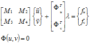
Where the u's are the dependent coordinates and the v's are the independent coordinates. The independent coordinates are not arbitrarily selected but chosen after performing a LU factorization of the constraint equations using full pivoting. The LU factorization will select the best choice of coordinates for the independent states.
The first step to exactly linearize the system is to define matrix P as:
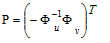
Multiplying the top row of the equations of motion by P and summing it to the second one, the Lagrange multipliers are eliminated:
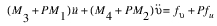 | (1) |
Differentiating the constraint equations one time we obtain:

A second differentiation returns:
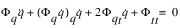
Partitioning the first term of the last equation we get:
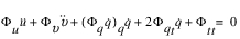
Rearranging this result we find:
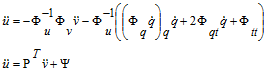
Putting this result into Equation (1), the ODE (minimal representation) of the equations of motion is found to be:

Notice that this equation has a functional dependency on both u and its first derivatives. However, both quantities can always be obtained from the constraint equations.
The final step is to perturb the ODE to obtain the linearized form:
 | (2) |
Adams Solver (C++) computes the equation above by using a different yet equivalent approach. Equation above is important because it shows that the contribution of each element can be singled out and exported. However, for the general dynamical case, the contribution of each element (inertial element, force or constraint) is heavily distributed all over the state matrices making very difficult the replacement of say an exported force by a new set of Nastran cards.
Approximate linearization
An approach followed by several computer codes consists of first linearizing the constraint equations, the equations motion and then assembling the ODE. The linearized constraints are:
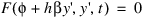 | (3) |
Redefining matrix P as
awe obtain that

Notice that in this case matrix P is numerically equal to matrix P defined in the previous section. However, in this case matrix P is a constant; therefore taking two time derivatives of the last expression we arrive to:
 | (4) |
The linearized equations of motion have this form:
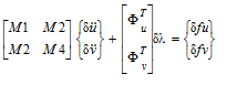 | (5) |
Multiplying the first row by P and summing it to the second row we find:
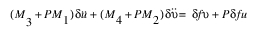
Combining this result with Equation (4) we arrive to:
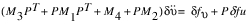 | (6) |
This is the set of assembled equations of motion obtained from the linearized constraint equations
(Equation (3)) and the linearized equations of motion (Equation (5)).
(Equation (3)) and the linearized equations of motion (Equation (5)).
Feasibility of the export approach
Comparing Equation (6) and Equation (2) we notice that, in the general case, eigenvalues computed by those two equations do not match. The complete variation of Equation (2) involves terms that are missing in Equation (2). (Notice that matrix P in Equation (6) is a constant.)
However, both Equation (6) and Equation (2) will produce the same eigenvalues only for the static case. If both velocities and accelerations are zero, several terms drop from Equation (2) and matching expressions are obtained except for the right-hand side (applied forces). The variation of the right-hand side on Equation (2) is:
which compared with the right-hand side of Equation (6) shows that there is a missing term a linear code can not compute. The solution is to export applied forces as DMIG cards.
Some of the issues addressed during the export job (OPENBOX option) are the following:
1. The linearization is internally performed using the same coordinates Nastran uses to assemble the equations of motion. This is accomplished by using Adams Solver (C++) capability to linearize the system in terms of user-defined coordinates.
2. The linearized constraint equations (Equation (3)) are evaluated by a two-stages process and exported a set of MPC cards.
3. The inertia elements (PARTS and POINT_MASS) are exported as CONM2 cards. This information is taken directly from a mass matrix obtained by temporarily deactivating all constraints. The mass matrices of flexible bodies are obtained in a similar way.
4. The stiffness and damping contribution of applied forces are computed and exported as DMIG cards. By default all forces and flexible bodies contributions are dumped into the same set of DMIGs. The configuration file can be used to single out the contribution of each applied force or flexible body, however, each singled out element involves one extra linearization.
5. All differential states contributions to the equations of motion are dumped into a set of DMIGs and SPOINT cards. Currently there are no tools to single out the contribution of differential states.
6. Examples
The command
LINEAR/EIGENSOL
computes an eigenanalysis for the Adams model. Adams Solver (C++) writes the eigenvalues and mode shapes to the Results file where they can be read and displayed by a postprocessor such as Adams View.
The command
LINEAR/STATEMAT, PINPUT=10, POUTPUT=20
, FORMAT=MATRIXX FILE=STATES.MAT
, FORMAT=MATRIXX FILE=STATES.MAT
computes state matrices for the Adams model, using PINPUT/10 as inputs and POUTPUT/20 as outputs. The state matrices are written to file STATES.MAT in MATRIXX format.
7. Applications
There are several areas in which the LINEAR command is required. Some examples include:
1. Eigensolutions provide you with information that may be used in assessing stability of the Adams model. If you import control systems descriptions or distributed elasticity data from external sources, you can verify the stability of their Adams models.
2. Eigendata computed by Adams Solver (C++) can be used to validate Adams models against eigendata from external sources.
3. State matrices descriptions can be used in designing control systems for Adams models. This description is suitable for computing frequency response data in matrix manipulation software packages (see the PINPUT, POUTPUT, and VARIABLE statements).
4. State matrices output by Adams Solver (C++) in the MATRIXX format are suitable for being read into a second Adams model with a MATRIX statement. These matrices can form the definition of a dynamical system defined by an LSE statement in the second Adams model.
5. Exported linearized model as Nastran bulk data decks using the "openbox" option can be used in eigensolutions, frequency response analysis using Nastran. The exported model can be further edited to perform other types of solution sequences in Nastran.
7.1 Eigen analysis application
Consider a model of an inverted pendulum on a sliding cart as shown in the figure shown next. The listing of the Adams Solver (C++) dataset for this model is shown in Listing 1 (see Appendix).
Figure 10 Inverted Pendulum on Sliding Cart Model
The sliding cart in this model is represented by PART/1 and the inverted pendulum is represented by PART/2. PART/1 slides along the global x axis in translational joint, JOINT/1, while PART/2 can rotate about the axis of revolute joint, JOINT/2. PART/1 is connected to ground by a SPRINGDAMPER/1. TFSISO/1 represents an actuator connected between PART/1 and PART/2. Force generated by this actuator is applied on the two parts by SFORCE/1. No input is applied to the actuator for the present. To assess stability of this model, execution of Adams Solver (C++) is initiated. Once Adams Solver (C++) verifies that the model data is syntactically correct, issue the SIMULATE/STATIC command. On achieving static equilibrium, issue the LINEAR/EIGEN command. Eigenvalues reported by Adams Solver (C++) are shown in the table below.
Model Eigenvalues
EIGENVALUES | ||
Number | Real (cycles/unit time) | Imag. (cycles/unit time) |
1 | 5.00909210E-02 | 0.00000000E+00 |
2 | -5.00924580E-02 | 0.00000000E+00 |
3 | -3.18309800E+01 | 0.00000000E+00 |
4 | -3.17994185E-01 | +/- 6.36188992E-01 |
The table shows that the system has three stable and one unstable mode. To determine the cause of this instability, use the data produced by Adams Solver (C++) (.res, .adm, and so on) in Adams to display the deformed mode shapes of the model.
Figure 11 (a) and (b) show mode shapes for mode 1, which is unstable, and mode 4, which is stable.
Figure 11 Deformed Mode Shape 4(a) and Deformed Mode Shape 4 (b)
Figure 11 (a) shows that PART/1 is essentially stationary while PART/2 is moving. You can conclude that PART/2 is the cause of the instability in this model. This is an expected result for this model, since the inverted pendulum is at an unstable operating point. It is obvious that disturbing the pendulum will cause it to swing about the revolute joint axis.
As illustrated by this example, viewing mode shapes in a graphical display can provide very significant insight into the dynamic behavior of the model. In complicated Adams models, this insight is vital in understanding the model dynamics. In Example 2: State Matrices Output below, based on the state matrices computed for this model, a feedback control law will be designed to stabilize this model.
7.2 State matrices output
This section presents the design and implementation of a control system for the Adams model described in Section 7.1. The purpose of the control design exercise is to design a feedback controller to attempt to stabilize the inverted pendulum. For control design purposes, the state matrix representation of the Adams model is required and is generated by the LINEAR/STATEMAT command.
Stabilization of this model requires that PART/2 maintain its inverted vertical position despite external disturbances applied on it. External disturbances considered here are gravity acting vertically downwards and an external force applied to the pendulum in the x-direction. On sensing a deviation of the pendulum from the desired position, the control law determines an appropriate signal to apply to actuator TFSISO/1 to restore PART/2 to its desired position. The control law operates on the basis of measuring output signals from the plant and then computes a signal to apply to the actuator.
As shown in Figure 12 for the present model, 3 signals are output by the plant. VARIABLE/10 is a measurement of the relative x displacement between PART/1 and PART/2. VARIABLE/20 is a measurement of the relative x velocities between the two parts. VARIABLE/30 is the integral of the relative x displacements between the two parts. These 3 signals are designated as outputs from the plant by POUTPUT/1.
Input to the plant, that is, input signal to the actuator, is defined as VARIABLE/2. This is designated as input to the plant by PINPUT/1. Adams Solver (C++) implementation of the input/output structure and the external disturbances is shown in Listing 2: Plant Input/output Specification (see Appendix). This implementation, when combined with the plant model as shown in dataset 1 in. This implementation, when combined with the plant model as shown in dataset 1 in FILE=c results in the open-loop model. When the open-loop model is complete, an Adams Solver (C++) execution session is initiated.
Figure 12 Open-Loop Model
The model is read into Adams Solver (C++). After Adams Solver (C++) verifies the model data syntax, issue the SIMULATE/STATIC command to determine the equilibrium position. On achieving the equilibrium position, issue the LINEAR/EIGEN, NOVECTOR command to verify the eigenvalues of the model. The next table shows the eigenvalues for the open-loop model.
Open-Loop Eigenvalues
EIGENVALUES | ||
Number | Real (cycles/unit time) | Imag. (cycles/unit time) |
1 | -2.66440631E-17 | 0.00000000E+00 |
2 | 5.00909210E-02 | 0.00000000E+00 |
3 | -5.00924580E-02 | 0.00000000E+00 |
4 | -3.18309800E+01 | 0.00000000E+00 |
5 | -3.17994185E-01 | +/- 6.36188992E-01 |
The table shows that the open-loop model has one eigenvalue more than the model in Eigenanalysis Application. This is due to the introduction of the relative displacement integrator TFSISO/2 in the open-loop model. To linearize the model and compute the state matrices, issue the LINEAR/STATEMAT, PINPUT=1, POUTPUT=1, file=adams.mat command. Adams Solver (C++) linearizes the model and writes the state matrices in the default format to adams.mat file. Contents of the ADAMS.MAT file are in Listing 3: State Matrices (FSAVE Format) for the Open-Loop Model (see Appendix). The Adams Solver (C++) session then terminates. You may design a controller by reading the ADAMS.MAT file into the control design package exercising various control design methodologies. The description of the control design step is beyond the scope of the present document. A text on this subject or documentation for control design software packages should be consulted for further details.
Now that the feedback control has been designed, it needs to be implemented in Adams Solver (C++) for a closed-loop simulation (see Listing 4 in the Appendix). The controller designed for this example is a dynamic compensator. As shown in Figure 13 below, this is implemented in Adams Solver (C++) as LSE/1. The A, B and C matrices associated with this LSE are defined by MATRIX/100, 200, and 300, respectively. Adams Solver (C++) reads the data for these matrices from a file named incomp.dat (see Listing 5 in the Appendix). To connect this feedback compensator to the plant model, inputs to LSE/1, ARRAY/303 are connected to outputs from the plant model. Also, ARRAY/1, which is input to the actuator, TFSISO/1, is now defined as the output from the compensator, VARIABLE/2. This completes the closed-loop Adams model. The complete Adams Solver (C++) dataset for this model Listing 4 (see Appendix).
Figure 13 Closed-Loop Model
To verify and simulate the closed-loop model, an Adams Solver (C++) simulation is initiated. The closed-loop model is first equilibrated in its static position. The eigenvalues for this model are computed and represented in Table 4 shown next.
Closed-Loop Eigenvalues
EIGENVALUES | ||
Number | Real (cycles/unit time) | Imag. (cycles/unit time) |
1 | -5.35233760E-01 | 0.00000000E+00 |
2 | -3.18270747E+01 | 0.00000000E+00 |
3 | -2.37397000E-01 | +/- 7.54488218E-02 |
4 | -7.37798519E-03 | +/- 1.51611302E-01 |
5 | -5.47796070E-01 | +/- 5.12745191E-01 |
6 | -2.43466412E-01 | +/- 5.71313964E-01 |
7 | -2.46528313E+01 | +/- 1.00614794E+01 |
Table 4 above shows that the closed-loop model is stable. The closed-loop model has more eigenvalues than the open-loop model. This is due to the dynamical state variables introduced by LSE/1. Eigenvalues for the closed-loop Adams model can be compared with the closed-loop eigenvalues computed in the control design package. Now that the stability properties of the closed-loop Adams model have been verified, it can be simulated to obtain its dynamic response. The time profile of the external disturbance is as shown in Figure 14. The closed-loop model response to external disturbance is as shown in Figure 15. As illustrated in this figure, the closed-loop model provides complete disturbance rejection for displacement of PART/2.
Figure 14 Time Profile of External Disturbance
Figure 15 Closed-Loop System Response
The input signal applied to the actuator and the force generated by the actuator are shown in Figure 16 and Figure 17, respectively.
Figure 16 Input Signal to Actuator
Figure 17 Force Generated by Actuator
The process of control design and simulation is an iterative one. If the closed-loop system does not perform as expected, the control design specifications may have to be changed and a new controller designed to achieve better performance.
8. Appendix
Listing 1: Inverted Pendulum Model
ADAMS Inverted pendulum model.
!
pa/99, ground
ma/99,qp=0,0,0, zp =1,0,0
!
! ===> Sliding cart <===
pa/1,ma=10,ip=10,10,10,cm=10
ma/10,qp=5,0,0 ! CM marker.
ma/11,qp=5,0,2, zp=5,1,2 ! revolute joint marker.
ma/12,qp=3,-2,-2 ! graphics marker.
ma/13,qp=5,0,0, zp=6,0,0 ! translational joint marker.
ma/14,qp=5,0,12
ma/15,qp=12,0,2 ! actutator attachment point
!
! ===> Inverted pendulum <===
pa/2,ma=1,cm=20, ip=1,1,1
ma/20,qp=5,0,12 ! CM marker.
ma/21,qp=5,0,2, zp=5,1,2 ! revolute joint marker.
ma/22,qp=5,0,12, zp=5,1,12 ! graphics marker.
ma/23,qp=5,0,7 ! actutator attachment point
ma/24,qp=5,0,2, zp=5,0,3 ! graphics marker.
!
joint/1,tran,i=13,j=99
joint/2,rev,i=11,j=21
!
! ===> Spring damper between cart and ground <===
springdamper/1,tran,i=99,j=13,k=200,c=40,l=5
!
gra/2, circle,cm=20, r=1.5,seg=20
gra/3, circle,cm=22, r=1.5,seg=20
gra/4, cylind,cm=24, l=8.5, r=0.25,seg=10,side=10
gra/5, box, corn=12, x=9, y=4, z=4
!
! ===> External disturbance <===
sforce/1001, i=20, j=99, action, tran,
,fun=step(time,0,0,.5,10)-step(time,1,0,1.5,10)
!
! ===>Actuator Dynamics<===
tfsiso/1,num=10, den=1,0.005
,u=1,x=2,y=3
array/1,u,var=2 ! input signal to actuator
array/2,x ! actuator state
array/3,y ! force generated by actuator.
!
! ===>Actuator force<===
sforce/1,i=15,j=23, trans,
,function=aryval(3,1)
!
! ===>Input to Actuator<===
vari/2,fun=0
!
accgrav/kg=-1
result/format
!
end
Listing 2: Plant Input/output Specification
! ===> PLANT INPUT/OUTPUT definition <===
! -------------------
!
var/1,fun=dx(20,14)
Displacement integrator
tfsiso/2, num=1, den=0,1
,u=20,x=21,y=22
array/20, U, VAR=1
array/21, X
array/22, Y
!
! ===> Outputs <===
vari/10, function= varval(1) ! displacement
vari/20, function= vx(20,14) ! velocity
vari/30, function= aryval(22,1) ! displ. integrated
!
!
! ===> Plant input designation <===
pinput/1,var=2
!
! ===> Plant output designation <===
poutput/1,var=10,20,30
!
Listing 3:State Matrices (FSAVE Format) for the Open-Loop Model
MATRIXx VERSION 700 7 2005-04-21 19:31:36
A 6 6B 6 1C 3 6D 3 1
STATES 3 6PINPUT 2 1POUTPUT 4 1
A 6 6 0(3(1PE25.17))
-3.99604352126607365e+00 1.00000000000000000e+00 3.95647873392680538e-01
0.00000000000000000e+00 0.00000000000000000e+00 0.00000000000000000e+00
-1.99802176063303669e+01 0.00000000000000000e+00 1.97823936696340263e+00
0.00000000000000000e+00 0.00000000000000000e+00 0.00000000000000000e+00
0.00000000000000000e+00 0.00000000000000000e+00 0.00000000000000000e+00
1.00000000000000000e+00 0.00000000000000000e+00 0.00000000000000000e+00
-9.89119683481701345e-02 0.00000000000000000e+00 1.08803165182987160e-01
0.00000000000000000e+00 0.00000000000000000e+00 1.00000000000000000e+01
4.02439896739235914e-02 0.00000000000000000e+00 -4.42683886413159505e-02
0.00000000000000000e+00 -2.00000000000000000e+02 0.00000000000000000e+00
0.00000000000000000e+00 0.00000000000000000e+00 0.00000000000000000e+00
0.00000000000000000e+00 0.00000000000000000e+00 0.00000000000000000e+00
B 6 1 0(3(1PE25.17))
0.00000000000000000e+00 0.00000000000000000e+00 0.00000000000000000e+00
0.00000000000000000e+00 2.00000000000000000e+03 0.00000000000000000e+00
C 3 6 0(3(1PE25.17))
0.00000000000000000e+00 0.00000000000000000e+00 0.00000000000000000e+00
0.00000000000000000e+00 0.00000000000000000e+00 0.00000000000000000e+00
0.00000000000000000e+00 1.00000000000000000e+01 0.00000000000000000e+00
1.00000000000000000e+01 0.00000000000000000e+00 0.00000000000000000e+00
0.00000000000000000e+00 0.00000000000000000e+00 0.00000000000000000e+00
0.00000000000000000e+00 0.00000000000000000e+00 1.00000000000000000e+00
D 3 1 0(3(1PE25.17))
0.00000000000000000e+00 0.00000000000000000e+00 0.00000000000000000e+00
STATES 3 6 0(3(1PE25.17))
2.10000000000000000e+01 1.00000000000000000e+00 7.00000000000000000e+00
2.10000000000000000e+01 1.00000000000000000e+00 1.00000000000000000e+00
2.10000000000000000e+01 2.00000000000000000e+00 1.10000000000000000e+01
2.10000000000000000e+01 2.00000000000000000e+00 5.00000000000000000e+00
3.00000000000000000e+00 1.00000000000000000e+00 1.00000000000000000e+00
3.00000000000000000e+00 2.00000000000000000e+00 1.00000000000000000e+00
PINPUT 2 1 0(3(1PE25.17))
1.00000000000000000e+00 2.00000000000000000e+00
POUTPUT 4 1 0(3(1PE25.17))
1.00000000000000000e+00 1.00000000000000000e+01 2.00000000000000000e+01
3.00000000000000000e+01
Listing 4: Closed-Loop Model
ADAMS Inverted pendulum closed-loop model.
!
pa/99, ground
ma/99,qp=0,0,0, zp =1,0,0
!
! ===> Sliding cart <===
pa/1,ma=10,ip=10,10,10,cm=10
ma/10,qp=5,0,0 ! CM marker.
ma/11,qp=5,0,2, zp=5,1,2 ! revolute joint marker.
ma/12,qp=3,-2,-2 ! graphics marker.
ma/13,qp=5,0,0, zp=6,0,0 ! translational joint marker.
ma/14,qp=5,0,12
ma/15,qp=12,0,2 ! actutator attachment point
!
! ===> Inverted pendulum <===
pa/2,ma=1,cm=20, ip=1,1,1
ma/20,qp=5,0,12 ! CM marker.
ma/21,qp=5,0,2, zp=5,1,2 ! revolute joint marker.
ma/22,qp=5,0,12, zp=5,1,12 ! graphics marker.
ma/23,qp=5,0,7 ! actutator attachment point
ma/24,qp=5,0,2, zp=5,0,3 ! graphics marker.
!
joint/1,tran,i=13,j=99
joint/2,rev,i=11,j=21
!
! ===> Spring damper between cart and ground <===
springdamper/1,tran,i=99,j=13,k=200,c=40,l=5
!
gra/2, circle,cm=20, r=2,seg=10
gra/3, circle,cm=22, r=2,seg=10
gra/4, cylind,cm=24, l=8, r=0.5,seg=10,side=10
gra/5, box, corn=12, x=9, y=4, z=4
!
! ===> External disturbance <===
sforce/1001, i=20, j=99, action, tran,
,fun=step(time,0,0,.5,10)-step(time,1,0,1.5,10)
!
! ===>Actuator Dynamics<===
tfsiso/1,num=10, den=1,0.005
,u=1,x=2,y=3
array/1,u,var=2 ! input signal to actuator
array/2,x ! actuator state
array/3,y ! force generated by actuator.
!
! ===>Actuator force<===
sforce/1,i=15,j=23, trans,
,function=aryval(3,1)
!
!
! ===> PLANT OUTPUT definition <===
! -------------------
!
var/1,fun=dx(20,14)
Displacement integrator
tfsiso/2, num=1, den=0,1
,u=20,x=21,y=22
array/20, u, var=1
array/21, x
array/22, y
!
! ===> Outputs <===
vari/10, function= varval(1) ! displacement
vari/20, function= vx(20,14) ! velocity
vari/30, function= aryval(22,1) ! displ. integrated
!
!
!
! ===> Plant output designation <===
poutput/1,var=10,20,30
!
! ===>Feedback compensator<===
! --------------------
!
lse/1,a=100, b=200, c=300,
,x=101,y=202,u=303,ic=404
!
array/101, x ! compensator state
array/202, y ! compensator output
array/303, u, var= 10, 20, 30 ! compensator input
array/404, ic, num=0,0,0,0,0,0
!
matrix/100,
,file=incomp.mat, name=ac
matrix/200,
,file=incomp.mat, name=bc
matrix/300,
,file=incomp.mat, name=cc1
!
! ===> Feedback signal from compensator to actuator <===
variable/2, fun=-aryval(202,1)
!
accgrav/kg=-1
result/format
!
End
Listing 5: "incomp.mat" Input Data file
MATRIXx VERSION 700 3 04-OCT-91 15:27
AC 6 6BC 6 3CC1 1 6
AC 6 6 0(1P3E25.17)
-1.00799962154710574E+01 9.75162440467575053E-01 9.98460749273361898E+01
9.61406957584617916E-01 3.11437948419828955E-03 -1.78574044858736743E+04
-8.50683303123077716E-01 -4.98921809045884790E-01 1.01587769607181722E+00
1.14325442554075640E+00 -4.49484043101296749E-01 -1.69576019090885748E+04
9.98009512743940519E+00 2.48375595324249708E-02 -9.98470640470196713E+01
3.85930424153820839E-02 -3.11437948419828955E-03 1.79036593612407414E+04
-1.48327577193440696E-01 4.98921809045884790E-01 -1.02576889290663420E+00
-1.14325442554075640E+00 4.49484043101296749E-01 1.74318979368853470E+04
-1.20450308829068348E-01 7.73595535159733033E-02 -1.23564688768258060E-01
-4.73156382486152438E-01 -1.34087821455120393E+00 2.82840625758381648E+04
4.02439896739235914E-02 0.00000000000000000E+00 -4.02439896739235858E-01
0.00000000000000000E+00 0.00000000000000000E+00 -2.09248210623341492E+02
BC 6 3 0(1P3E25.17)
1.38436380363864547E-01 -4.98921809064772792E-01 1.12468086129738198E+00
1.14325442558403734E+00 5.50515956881686863E-01 -9.30005800767228163E-01
-9.98009512743940519E+00 -2.48375595324249708E-02 9.98470640470196713E+01
9.61406957584617916E-01 3.11437948419828955E-03 -1.36246052474731605E+04
1.20450308829068348E-01 -7.73595535159733033E-02 1.23564688768258060E-01
4.73156382486152438E-01 1.34087821455120393E+00 2.08671855656208993E-01
CC1 1 6 0(1P3E25.17)
2.11639961920025588E+00 8.47833595164392051E+00 -2.13952705688378986E+00
-8.71548396554230820E+00 -1.41421356238469098E+01 4.62410531167074812E-03
Listing 6: Input data file used in Section Differences in results compared with Adams Solver FORTRAN
Adams View model name: MODEL_1
!
UNITS/
, FORCE = NEWTON
, MASS = KILOGRAM
, LENGTH = MILLIMETER
, TIME = SECOND
!
! adams_view_name='ground'
PART/1
, GROUND
!
! adams_view_name='MARKER_4'
MARKER/4
, PART = 1
, QP = 0, 400, 0
!
! adams_view_name='MARKER_6'
MARKER/6
, PART = 1
, QP = 300, 350, 0
!
! adams_view_name='MARKER_9'
MARKER/9
, PART = 1
, QP = 300, 400, 0
!
! adams_view_name='BOX_6'
GRAPHICS/6
, BOX
, CORNER = 9
, X = 150
, Y = -250
, Z = 300
!
! adams_view_name='PART_2'
PART/2
, MASS = 2.945180253
, CM = 7
, IP = 48894.82242, 48589.74352, 513.6958387
!
! adams_view_name='MARKER_1'
MARKER/1
, PART = 2
, QP = 0, 400, 0
, REULER = 284.0362435D, 0D, 0D
!
! adams_view_name='MARKER_3'
MARKER/3
, PART = 2
, QP = 0, 400, 0
!
! adams_view_name='MARKER_5'
MARKER/5
, PART = 2
, QP = 50, 200, 0
!
! adams_view_name='cm'
MARKER/7
, PART = 2
, QP = 50, 200, 0
, REULER = 194.0362435D, 90.00000002D, 90.00000017D
!
! adams_view_name='MARKER_10'
MARKER/10
, PART = 2
, QP = -50, 400, 0
!
! adams_view_name='BOX_7'
GRAPHICS/7
, BOX
, CORNER = 10
, X = 100
, Y = -350
, Z = 200
! adams_view_name='SPRING_1.I_graphic'
GRAPHICS/1
, FORCE
, ETYPE = SFORCE
, EID = 1
, EMARKER = 5
!
! adams_view_name='SPRING_1.J_graphic'
GRAPHICS/2
, FORCE
, ETYPE = SFORCE
, EID = 1
, EMARKER = 6
!
! adams_view_name='SPRING_1.spring_graphic'
GRAPHICS/3
, SPDP
, I = 5
, J = 6
, COILS = 10
, DA = 58.30951895
!
! adams_view_name='SPRING_1.damper_graphic'
GRAPHICS/4
, SPDP
, I = 5
, J = 6
, COILS = 0
, DB = 29.15475947
, DC = 23.32380758
, LC = 195.3368885
, LD = 195.3368885
!
! adams_view_name='JOINT_1'
JOINT/1
, REVOLUTE
, I = 3
, J = 4
!
! adams_view_name='SPRING_1.sforce'
SFORCE/1
, TRANSLATIONAL
, I = 5
, J = 6
, FUNCTION = - 1.2E-002*(DM(5,6)-291.5475947423)
, - 2.9E-003*VR(5,6)
, + 0.0
!
! adams_view_name='SPRING_1.deformation'
VARIABLE/1
, FUNCTION = DM(5,6) - 291.5475947423
!
! adams_view_name='SPRING_1.deformation_velocity'
VARIABLE/2
, FUNCTION = VR(5,6)
!
! adams_view_name='SPRING_1.force'
VARIABLE/3
, FUNCTION = (DX(5,6)*FX(5,6) +
, DY(5,6)*FY(5,6) +
, DZ(5,6)*FZ(5,6))/
, DM(5,6)
!
! adams_view_name='VARIABLE_5'
VARIABLE/5
, FUNCTION = DX(7)
!
! adams_view_name='PSTATE_1'
PSTATE/1
, VARIABLES = 5
!
ACCGRAV/
, JGRAV = -9806.65
!
RESULTS/
, XRF
!
END
Listing 7: Adams Solver FORTRAN command file used in section Differences in results compared with Adams Solver FORTRAN.
model_1
F77
preferences/solver=f77
SIMULATE/STATIC
LINEAR/EIGENSOL, ENERGY=1, DISSIPAT=1, KINETIC=1, STRAIN=1
Stop
Listing 8: Adams Solver C++ command file used in Section Differences in results compared with Adams Solver FORTRAN.
model_1
CxxNoPstate
SIMULATE/STATIC
LINEAR/EIGENSOL, ENERGY=1, DISSIPAT=1, KINETIC=1, STRAIN=1
stop
Listing 9: Adams Solver C++ command file used in Section Differences in results compared with Adams Solver FORTRAN using PSTATE.
model_1
CxxYesPstate
SIMULATE/STATIC
LINEAR/EIGENSOL, ENERGY=1, DISSIPAT=1, KINETIC=1, STRAIN=1, PSTATE=1
stop
9. Limitations
■Although Adams Solver C++ has a sound implementation of a linearization algorithm, it does have limitations. One such limitation is related to very stiff systems. The process to assemble the linearization matrix requires the solution of an enormous system of equations. If your system is too stiff (large disproportion of stiffness elements), the solution process is affected and the quality of the obtained matrix may be degraded.
■Another limitation is related to large models. Currently in standard hardware configurations running Windows 7 with 8G RAM, the limit appears to be between 20,000 and 30,000 degrees-of-freedom. Such large models can't be linearized due to memory addressing issues. This limitation will be removed in future releases.
■Models with GCONs defining velocity constraints can't be linearized. This limitation will also be removed in future releases.
■Notice that an implicit algebraic DIFF does not create a differential equation in the model, in fact they are equivalent to a variable definition. For instance,
DIFF/4, IMPLICIT, FUNCTION=DIF(4)-TIME*DX(777)
is such a case because the above FUNCTION definition makes no use of the expression DIF1(4) (the time derivative of the state), only DIF(4) is used (the plain value of the state). Implicit algebraic DIFFs are usually defined with the purpose to obtain the time derivative of an expression. For example, DIF1(4) will in fact return the time derivative of the expression TIME*DX(777) for the above statement. However, the time derivative in this case is compute numerically as a byproduct of the numerical integration. Hence, using the expression DIF1(4) in a force definition will produce wrong linearization results because the partial derivatives of the time derivative DIF1(4) with respect to the states of the system will return a zero value. Adams Solver C++ does not have an expression for DIF1(4) that can be used to compute the required partial derivatives.
See other Simulation available.