System Elements
System elements allow you to add your own algebraic and differential equations, and corresponding states, to your model. Adams Solver solves your equations simultaneously with the equations it generates from other modeling elements.
Your user-defined equations can depend on any states in the model, such as time, part motions, forces, or other user-defined states. In turn, you can reference your states in forces, system elements, and other modeling elements.
System elements enable you to model system components that are not as easily represented by standard Adams View modeling objects, such as parts, constraints, and forces. They are useful for modeling components or subsystems that have dynamics of their own. You can use system elements to represent a control system, for example, or to model the dynamics of an electro-mechanical, hydraulic, or pneumatic actuator. You can also use system elements to compute simulation output. For example, you might calculate the energy dissipated in a damper.
The system elements are listed in the table below.
The system element: | Defines: |
|---|---|
Differential equation that describes a user-defined variable in terms of its time derivative. | |
System of explicit differential and (optionally) algebraic equations in state-space form. You use array data elements to specify inputs, outputs, and statements. | |
System of constant coefficient, explicit, differential, and algebraic equations in the classic state-space format when used with associated array and matrix data elements. | |
Single-input, single-output transfer function as a ratio of two polynomials in the Laplace domain when used with associated array data elements. | |
Scalar algebraic equation for independent use or as part of the plant input, plant output, or array data elements. |
Example of Using System Element
We've provided a complete example of using System elements in a model in the examples directory of your Adams installation directory. The example contains the following elements:
The files you use to run the example are:
■system_tutorial.cmd - Contains an Adams View command file that builds a model containing the elements listed above.
■system_tutorial.txt - Describes the model and its construction.
The path to the files is /install_dir/aview/examples/user_guide, where install_dir is where the Adams software is installed.
Controlling Equilibrium Values When Using System Elements
During a static simulation, Adams Solver finds equilibrium values for user-defined differential variables (differential equations, general state equations, linear state equations, and transfer functions), as well as for the displacement and force variables. The equilibrium values it finds change the initial conditions for subsequent simulations. To help you control the static simulation results, Adams View provides an option that you can set to keep the values constant. This option is called static hold. Static hold retains the user-specified initial conditions as the static equilibrium values.
If you do not set static hold, Adams Solver sets the time derivatives of the user-defined variables to zero during a static simulation, and uses the user-supplied initial-condition values only as initial guesses for the static solution. Generally, the final equilibrium values are not the same as the initial condition values. Adams Solver then uses the equilibrium values of the user-defined variables as the initial values for any subsequent simulation, just as with the equilibrium displacement and force values.
If you do set static hold, Adams Solver retains the user-specified initial conditions as the static equilibrium values. Therefore, the final equilibrium values are the same as the user-specified initial conditions. Note that this does not guarantee that the time derivatives of the user-defined variable are zero after a static simulation.
Using Arrays with System Elements
You use array elements to represent the system states and outputs for linear state equations, general state equations, and transfer functions. You use the run-time function ARYVAL to reference states and outputs for these elements, instead of using Adams functions that are dedicated expressly to the equations. For more information on arrays, see Creating and Modifying Arrays. For more information on the ARYVAL function, see Adams View Function Builder online help.
The state variable and differential equation elements do not use arrays. You reference a state variable with the VARVAL function, and reference a differential equation with the DIF and DIF1 functions. Again, for more information on these functions, see Adams View Function Builder online help.
Terminology Used in System Elements
The terminology used in the dialog boxes for creating linear state equations, general state equations, and transfer function follows standard control systems terminology, where:
■x is the state array
■y is the output array
■u is the input array
■IC is the initial conditions array, x(t=0)
You define each of these arrays using an array data element stored in the current Modeling database. All array sizes must be consistent with the definition of the system elements. Do not define arrays with zero-size and zero-valued partial-derivative matrices. Adams Solver correctly formulates the system equations based on those arrays and derivatives that do exist.
About Using Differential Equations
A differential equation creates a user-defined state variable and defines a first-order differential equation that describes it. The equation can be dependent on any Adams Solver state variable available in a function expression except Point-Curve Constraints and 2D Curve-Curve Constraints. You can create systems of differential equations using more than one differential equation, linear state equation, or general state equation.
You describe the variable in a differential equation either by writing a function expression or User-written subroutine. Because it is easier to write function expressions than subroutines, you should use function expressions whenever possible to describe user-defined differential variables.
Ways to Define Differential Equations
You can define the differential equation in either explicit or implicit form. The following equation defines the explicit form of a differential equation:
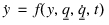
where:
■ is the time derivative of the user-defined state variable.
is the time derivative of the user-defined state variable.■y is the user-defined state variable itself.
 is a vector of
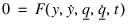
 You need to use the implicit form if the first derivative of the state variable cannot be isolated. The following equation defines the implicit form of a differential equation:
Ways You Can Use Differential Equations
Differential equations are best for creating single equations or small sets of equations. Although you can create sets of differential equations to represent higher-order equations or large systems of equations, other Adams Solver elements, such as transfer functions, linear state equations, or general state equations, can be more convenient in these cases.
You can use the solution to the differential equation in function expression that define a number of other elements in Adams, such as a force, or in User-written subroutines. Both function expressions and user-written subroutines can access the user-defined state variable and its derivative. Therefore, you can use Adams Solver to solve an independent initial value problem, or you can fully couple the differential equations with the system of equations that governs the dynamics of the problem.
Function expressions access the state variable using the function DIF(i1) and the derivative using DIF1(i1). In each case, i1 specifies the name of the differential equation that defines the variable. User-written subroutines access the value and derivative by calling the subroutine SYSFNC. For more information on functions, see Adams View Function Builder online help. For more information on subroutines, see the Subroutines section of the Adams Solver online help.
Creating and Modifying Differential Equation
The following procedure explains how to create or modify a differential equation.
To create or modify differential equations:
1. Click the Elements tab. From the System Elements container, click the Differential Equation tool .
.
. or
(Classic interface) From the Build menu, point to System Elements, point to Differential Equation, and then select either New or Modify.
2. If you selected Modify, the Database Navigator appears. Select a differential equation to modify.
The Create/Modify Differential Equation dialog box appears. Both dialog boxes contain the same options.
3. If you selected New, change the name of the differential equation element, if desired.
4. Set Type to either Explicit or Implicit to indicate that the function expression or User-written subroutine defines the explicit or implicit form of the equation. Learn about Ways to Define Differential Equations.
5. Do either of the following:
■Set Definition to Run-time Expression, and, in the y' = text box, enter a function expression that Adams Solver evaluates during a Simulation. In the function expression, the system variable DIF(i) is the value of the dependent variable that the differential equation defines, and DIF1(j) is the first derivative of the dependent variable that the differential equation defines.
Select the More button  to display the Function Builder and build an expression. See Function Builder and Adams View Function Builder online help.
to display the Function Builder and build an expression. See Function Builder and Adams View Function Builder online help.■Set Definition to User Written Subroutine and in the y' = text box, enter parameters that are passed to a user-written subroutine DIFSUB or specify an alternative library and name for the user subroutine in the Routine text box. Learn about Adams Solver Subroutines. Learn about specifying routines with ROUTINE Argument.
6. In the Initial Conditions text box, specify:
■The initial value of the differential equation at the start of the simulation.
■Optionally, if you are defining an implicit equation, an approximate value of the initial time derivative of the differential equation at the start of the simulation. (You do not need to supply a second value when you enter a explicit equation because Adams Solver can compute the initial time derivative directly from the equation.)
7. Adams Solver might adjust the value of the time derivative when it performs an initial conditions simulation. Entering an initial value for the time derivative helps Adams Solver converge to a desired initial conditions solution.
8. Select whether or not Adams should hold constant the value of the differential equation during static and quasi-static Simulations. Learn about Controlling Equilibrium Values When Using System Elements.
Creating and Modifying General State Equations
The following procedure teaches you how to represent a subsystem that has well defined inputs (u), internal states (x), and a set of well defined outputs (y).
See GSE statement in the Adams Solver online help for an extensive discussion on General State equations.
To create or modify a general state equation:
1. Click the Elements tab. From the System Elements container, click the General State Equation tool .
.
. or
(Classic interface) From the Build menu, point to System Elements, point to General State Equation, and then select either New or Modify.
2. If you selected Modify, the Database Navigator appears. Select a system element to modify.
The Create/Modify General State Equation dialog box appears. Both dialog boxes contain the same options.
3. If you selected New, change the name of the general state equation element, if desired, and assign a unique ID to it.
4. Set up the GSE by filling in the following text boxes:
■In the U Array (Inputs) text box, specify the array element that defines the input variables for the GSE. The U array is optional. When not specified, there are no system inputs. The number of inputs to the GSE is inferred from the number of variables in the U array.
■In the Y Array (Outputs) text box, specify the array element that defines the output variables for the GSE.
■In the User Function Parameters text box, specify the parameters that are to be passed to the User-written subroutines that define the constitutive equations of a GSE, viz., Equations (1), (2), and (3).
Three user subroutines are associated with a GSE:
♦GSE_DERIV is called to evaluate fc() in Equations 1.
♦GSE_UPDATE is called to evaluate fd() in Equations 2.
♦GSE_OUTPUT is called to evaluate g() in Equations 3.
See the Subroutines help in the Adams Solver online help.
If you specified a user function, in the Interface Function Names, enter function names to use other than the standard names GSE_DERIV, GSE_UPDATE, and GSE_OUTPUT.
5. Set States to the type of system to define:
■None (No options appear; defines a Feed-Forward Only System)
The dialog box changes depending on the type of system. See the next tables for the values to enter depending on the systems you are creating. For a sampled system, you enter both continous and discrete values.
6. Add or change any comments about the GSE that you want to enter to help you manage and identify it.
7. Select OK.
Options for Defining Continuous and Sampled Systems
For the option: | Do the following: |
|---|---|
X Array (Continous) | Enter the array element that defines the continuous states for the GSE. The array element must be of the X type, and it cannot be used in any other linear state equation, general state equation, or transfer function. |
IC Array (Continous) | Enter the array element that specifies the initial conditions for the continuous states in the system. When you do not specify an IC array for a GSE, all the continuous states are initialized to zero. |
Static Hold | Indicate whether or not the continuous GSE states are permitted to change during static and quasi-static simulations. |
Options for Discrete and Sampled Systems
For the option: | Do the following: |
|---|---|
X Array (Discrete) | Enter the array element that is used to access the discrete states for the GSE. It must be of the X type, and it cannot be used in any other linear state equation, general state equation, or transfer function. |
IC Array (Discrete) | Enter the array element that specifies the initial conditions for the discrete states in the system. The array is optional. The array element must be of the IC type. When you do not specify an IC array for a GSE, all the discrete states are initialized to zero. |
First Sample Time | Specify the Simulation time at which the sampling of the discrete states is to start. All discrete states before the first sample time are defined to be at the initial condition specified. The default is zero. |
Sample Function/Sample User Parameters | Specify the sampling period associated with the discrete states of a GSE. This tells Adams Solver to control its step size so that the discrete states of the GSE are updated at: last_sample_time + sample_period In cases where an expression for the sampling period is difficult to write, you can specify it in a user-written subroutine GSE_SAMP. Adams Solver will call this function at each sample time to find out the next sample period. Select the More button to display the Function Builder and build an expression. See Function Builder and Adams View Function Builder online help. |
Creating and Modifying Linear State Equations
The following procedure explains how to create a linear state equation.
See LSE statement in Adams Solver online help for an extensive discussion on Linear State Equations.
To create or modify a linear state equation:
1. Click the Elements tab. From the System Elements container, click the Linear State Equation tool .
.
. or
(Classic interface) From the Build menu, point to System Elements, point to Linear State Equation, and then select either New or Modify.
2. If you selected Modify, the Database Navigator appears. Select a linear state equation to modify.
The Part Create Equation Linear State Equation or Part Modify Equation Linear State Equation dialog box appears. Both dialog boxes contain the same options.
3. If you selected New, change the name of the linear state equation element, if desired, and assign a unique ID number to it.
4. Add or change any comments about the equation element that you want to enter to help you manage and identify the element.
5. Enter the arrays and matrices in the next text boxes as explained below.
■X State Array Name - Enter the array element that defines the state array for the linear system. The array must be a states (X) array. It cannot be used in any other linear state equation, general state equation, or transfer function.
■U Input Array Name - Enter the array element that defines the input (or control) array for the linear system. Entering an inputs (U) array is optional. The array must be an inputs (U) array. If you enter an inputs (U) array, you must also specify either a B input matrix, a D feedforward matrix, or both.
The B and D matrices must have the same number of columns as there are elements in the inputs (U) array.
■Y Output Array Name - Enter the array element that defines the column matrix of output variables for the linear system. Entering an outputs (Y) array is optional. If you enter an outputs (Y) array, you must also specify a C output matrix or a D feedforward matrix. The corresponding matrix elements must have the same number of rows as there are elements in the outputs (Y) array. It also must be an outputs (Y) array, and it cannot be used in any other linear state equation, general state equation, or transfer function.
■IC Array Name - Enter the array element that defines the column matrix of initial conditions for the linear system. Entering the IC array is optional. The IC array must have the same number of elements as the states (X) array (equal to the number of rows in the A state matrix). When you do not specify an IC array, Adams Solver initializes all states to zero.
■A State Matrix Name - Enter the matrix data element that defines the state transition matrix for the linear system. The matrix must be a square matrix (same number of rows and columns), and it must have the same number of columns as the number of rows in the states (X) array.
■B Input Matrix Name - Enter the matrix data element that defines the control matrix for the linear system. The B input matrix must have the same number of rows as the A state matrix and the same number of columns as the number of elements in the inputs (U) array.
Entering a B input matrix is optional. If you enter a B input matrix, you must also include an inputs (U) array.
■C Output Matrix Name - Enter the matrix data element that defines the output matrix for the linear system. The C output matrix must have the same number of columns as the A state matrix and the same number of rows as the number of elements in the outputs (Y) array. Entering a C output matrix is optional. If you enter a C output matrix, you must also include an outputs (Y) array name.
■D Feedforward Matrix Name - Enter the matrix data element that defines the feedforward matrix for the linear system. The D feedforward matrix must have the same number of rows as the number of elements in the Y output array and the same number of columns as the number of elements in the inputs (U) array.
When you enter a D feedforward matrix, you must also include both a Y output matrix and an inputs (U) array.
6. Set Static hold to yes to hold states at the constant value determined during static and quasi-static simulations; no if they can change. Learn about Controlling Equilibrium Values When Using System Elements.
7. Select OK.
Creating and Modifying Transfer Functions
The following procedure examples how to create or modify a transfer function.
See TFSISO statement in Adams Solver online help for an extensive discussion on Transfer functions.
To create or modify a transfer function:
1. Click the Elements tab. From the System Elements container, click the Transfer Function tool .
.
or
(Classic interface) From the Build menu, point to System Elements, point to Transfer Function, and then select either New or Modify.
3. The Create/Modify Transfer Function dialog box appears. Both dialog boxes contain the same options.
4. If you selected New, change the name of the transfer function element, if desired.
5. Enter the arrays for the transfer function in the next three text boxes as explained below:
■Input Array Name (U) - Enter the array that defines the input (or control) for the transfer function. The array must be an inputs (U) array. If you specified the size of the array when you created it, it must be one.
■State Array Name (X) - Enter the array that defines the state variable array for the transfer function. The array must be a states (X) array, and it cannot be used in any other linear state equation, general state equation, or transfer function. If you specified the size of the array when you created it, it must be one less than the number of coefficients in the denominator.
■Output Array (Y) - Enter the array that defines the output for the transfer function. The array must be an outputs (Y) array, and it cannot be used in any other linear state equation, general state equation, or transfer function. If you specify the size of the array when you created it, its size must be one.
6. In the Denominator Coefficients and Numerator Coefficients text boxes, specify the coefficients of the polynomial in the numerator and denominator of the transfer function. List the coefficients in order of ascending power of s, starting with s to the zero power, including any intermediate zero coefficients. The number of coefficients for the denominator must be greater than or equal to the number of coefficients for the numerator. The number of coefficients for the denominator must be greater than or equal to the number of coefficients for the numerator.
7. Select Check Format and Display Plot to display a plot of the transfer function. (see Plots Transfer Function dialog box help)
8. Select whether or not Adams should hold constant the value of the transfer equation during static and quasi-static Simulations. Learn about Controlling Equilibrium Values When Using System Elements.
9. Select OK.
About State Variables
You create state variables to define scalar algebraic equations for independent use or as part of the plant input, plant output, or array elements. The computed value of the variable can depend on almost any Adams system variable. Note that you cannot access reaction forces from Point-Curve Constraints and Curve-Curve Constraints.
You use state variables in the following ways:
■With plant input and plant output elements to identify inputs and output for an Adams Linear solution. For information on using Adams Linear and plant inputs and plant outputs, see the Adams Solver online help.
■With array elements to identify inputs to linear state equations, general state equations, and transfer functions.
■Independently to break up long function expressions into several parts or to compute common values that you need in several other function expressions. Using state variables to compute intermediate values can make complex expressions easier to read and modify. If you use the expression in many places, computing it once in a state variable can also be faster computationally.
Ways to Define State Variables
You can define the computed value of a variable by either:
■Writing a function expression in the model.
Function expressions and user-written subroutines can access the computed value of the variable using the Adams View function VARVAL(variable_name) to represent the value, where variable_name specifies the name of the variable. User-written subroutines access a single variable by calling the subroutine SYSFNC.
For more information on functions, see Adams View Function Builder online help. For more information on subroutines, see the Subroutines section of the Adams Solver online help.
Cautions When Using State Variables
You should use caution when defining variables that are dependent on other variables or on Adams View elements that contain functions. It is possible to create equations that cannot be solved. If a defined system of equations does not have a stable solution, convergence can fail for the entire Adams model.
For example, if you define your state variable my_variable using the function expression:
F = varval(my_variable) + 1
You are defining the following algebraic equation that has no solution:
V = V + 1
When Adams Solver tries to solve this equation using the Newton-Raphson iteration, the solution diverges and a message appears on the screen indicating that the solution has failed to converge.
Creating and Modifying State Variables
The following procedure explains how to create or modify a state variable.
To create and modify a state variable:
1. Click the Elements tab. From the System Elements container, click the State Variable tool .
.
. or
(Classic interface) From the Build menu, point to System Elements, point to State Variable, and then select either New or Modify.
The Create/Modify State Variable dialog box appears.
3. If you selected New, change the name of the state variable element, if desired
4. Set Definition to either of the following:
■Run-time Expression
■User written subroutine
Learn more about Ways to Define State Variables.
5. If you selected:
■Run-time Expression, enter the function expression that defines the variable. Select the More button to display the Function Builder and build an expression. See Function Builder and Adams View Function Builder online help.
to display the Function Builder and build an expression. See Function Builder and Adams View Function Builder online help.■User written subroutine, enter constants to the User-written subroutine VARSUB to define a variable. See the Subroutines section of the Adams Solver online help.
6. If desired, select Guess for F(1, 0..), and then specify an approximate initial value for the variable. Adams Solver may adjust the value when it performs an Initial conditions simulation. Entering an accurate value for initial conditions can help Adams Solver converge to the initial conditions solution.