Flexible Connectors
Bushings
Creating Bushings
To define a bushing, you need to create two markers, one for each part. The marker on the first part that you specify is called the I marker. The marker on the second part that you specify is called the J marker.
Learn about Constitutive Equations for Bushings.
To create a bushing:
 .
. 2. In the settings container, specify the following:
■How you want the force applied to parts. You can select the following:
♦1 Location
♦2 Bodies - 1 Location
♦2 Bodies - 2 Locations
Learn about Applying Multi-Component Forces to Parts.
■How you want the force oriented. You can select:
♦Normal to Grid - Lets you orient the force using the x-, y-, and z-axes of the current Working grid, if it is displayed, or using the x-, y, and z-axes of the screen.
♦Pick Feature - Lets you orient the force along a direction vector on a feature in your model, such as the face of a part. The direction vector you select defines the z-axis for the force; Adams View automatically calculates the x- and y-axes.
■The translational and rotational stiffness and damping properties for the bushing.
3. Click the bodies.
4. Click one or two force-application points depending on the location method you selected.
5. If you selected to orient the force along a direction vector using a feature, move the cursor around in your model to display an arrow that shows the direction along a feature where you want the force oriented. Click when the direction vector shows the correct z-axis orientation.
Modifying Bushings
The following procedure modifies the following for a Bushing:
■The two bodies to which the forces are applied.
■Translational and rotational properties for stiffness, damping, and preload.
Learn about Constitutive Equations for Bushings.
To modify a bushing:
2. Enter the values in the dialog box as explained the table below, and then select OK.
To: | Do the following: |
|---|---|
Tips on Entering Object Names in Text Boxes. | |
Set the bodies used in defining the force | Change the following as necessary in the following text boxes. The text boxes available depend on how you defined the direction of the force. ■Action Body - Change the action body to which the force is applied. ■Reaction Body - Change the body that receives the reaction forces. |
Change the properties of the force | For the translational force applied by the bushing, enter: ■Three stiffness coefficients. ■Three viscous-damping coefficients. The force due to damping is zero when there are no relative translational velocities between the markers on the action and reaction bodies. ■Enter three constant force (preload) values. Constant values indicate the magnitude of the force components along the x-, y-, and z-axeis of the coordinate system marker of the reaction body (J marker) when both the relative translational displacement and velocity of the markers on the action and reaction bodies are zero. For the rotational (torque) properties, enter: ■Three stiffness coefficients. ■Three viscous-damping coefficients. The torque due to damping is zero when there are no relative rotational velocities between the markers on the action and reaction bodies. ■Three constant torque (preload) values. Constant values indicate the magnitude of the torque components about the x-, y-, and z-axes of the coordinate system marker on the reaction body (J marker) when both the relative rotational displacement and velocity of the markers on the action and reaction bodies are zero. |
Set force graphics | Set Force Display to whether you want to display force graphics for one of the parts, both, or none. |
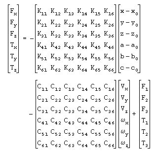
Constitutive Equations for Bushings
The following constitutive equations define how Adams View uses the data for a linear Bushing to apply a force and a torque to the action body depending on the displacement and velocity of the I marker on the action body relative to the J marker on the reaction body.
Note: | A bushing has the same constitutive relation form as a field element. The primary difference between the two forces is that non diagonal coefficients (Kij and Cij, where i is not equal to j) are zero for a bushing. You only define the diagonal coefficients (Kii and Cii) when creating a bushing. For more on field elements, see Field Element Tool. |
where:
■Fx, Fy, and Fz are measure numbers of the translational force components in the coordinate system of the J marker.
■x, y, and z are measure numbers of the bushing deformation vector in the coordinate system of the J marker.
■Vx, Vy, and Vz are time derivatives of x, y, and z, respectively.
■F1, F2, and F3 are measure numbers of any constant preload force components in the coordinate system of the J marker.
■Tx, Ty, and Tz are rotational force components in the coordinate system of the J marker.
■a, b, and c are projected, small-angle rotational displacements of the I marker with respect to the J marker.
■wx, wy, and wz are the measure numbers of the angular velocity of the I marker as seen by the J marker, expressed in the J marker coordinate system.
■T1, T2, and T3 are measure numbers of any constant preload torque components in the coordinate system of the J marker.
The bushing element applies an equilibrating force and torque to the J marker in the following way:
where:
■ is the instantaneous deformation vector from the J marker to the I marker. While the force at the J marker is equal and opposite to the force at the I marker, the torque at the J marker is usually not equal to the torque at the I marker because of the moment arm due to the deformation of the bushing element.
is the instantaneous deformation vector from the J marker to the I marker. While the force at the J marker is equal and opposite to the force at the I marker, the torque at the J marker is usually not equal to the torque at the I marker because of the moment arm due to the deformation of the bushing element.For the rotational constitutive equations to be accurate, at least two of the rotations (a, b, c) must be small. That is, two of the three values must remain smaller than 10 degrees. In addition, if a becomes greater than 90 degrees, b becomes erratic. If b becomes greater than 90 degrees, a becomes erratic. Only c can become greater than 90 degrees without causing convergence problems. For these reasons, it is best to define your bushing such that angles a and b remain small (not a and c and not b and c).
Advanced Bushings
Advanced bushing supports two modeling methods.
1. General Bushing
2. Nonlinear Bushing
To define a bushing, you need to create two markers, one for each part. The marker on the first part that you specify is called the I marker. The marker on the second part that you specify is called the J marker.
To create an advance bushing:
1. From the Create Forces tool stack or palette, select either General Bushing or Nonlinear BushingsTool  .
.
. 2. In the settings container, specify the following:
■How you want the force applied to parts. You can select the following:
♦1 Location
♦2 Bodies - 1 Location
♦2 Bodies - 2 Locations
Learn about Applying Multi-Component Forces to Parts.
■How you want the force oriented. You can select:
♦Normal to Grid - Lets you orient the force using the x-, y-, and z-axes of the current Working grid, if it is displayed, or using the x-, y, and z-axes of the screen.
♦Pick Feature - Lets you orient the force along a direction vector on a feature in your model, such as the face of a part. The direction vector you select defines the z-axis for the force; Adams View automatically calculates the x- and y-axes.
■General bushing property file (accepts .gbu file, default file located at <top_dir>/aview/examples/bushings)
■Nonlinear bushing property file (accepts .bus file, default file located at <top_dir>/aview/examples/bushings)
3. Click the bodies.
4. Click one or two force-application points depending on the location method you selected.
5. If you selected to orient the force along a direction vector using a feature, move the cursor around in your model to display an arrow that shows the direction along a feature where you want the force oriented. Click when the direction vector shows the correct z-axis orientation.
Modifying Advanced Bushings
The following procedure modifies the following for a Bushing:
■The two bodies to which the forces are applied.
■Bushing icon geometry (length and radius)
■Linear/Torsional preloads
■Linear/Torsional offsets
■General Bushing property file
To modify a general bushing:
2. Enter the values in the dialog box as explained the table below, and then select OK.
To: | Do the following: |
|---|---|
Set the bodies used in defining the force | Change the following as necessary in the following text boxes. The text boxes available depend on how you defined the direction of the force. ■Action Body - Change the action body to which the force is applied. ■Reaction Body - Change the body that receives the reaction forces. |
Geometry | Enter length/radius for bushing icon geometry |
Set force graphics | Set Force Display to whether you want to display force graphics for one of the parts, both, or none. |
Change the properties of the force | For linear/rotational preloads/offsets, enter: ■Three preload real values. ■Three offset real values. |
Property File | Accepts a bushing property file *.bus for nonlinear bushing and *.gbu for general bushing For more details of general bushing property file contents please refer to General Bushing. For more details of nonlinear bushing property file contents please refer to Nonlinear Bushings. |
To learn about bushings click on the below links.
Translational Spring Dampers
A translational spring damper represents forces acting between two parts over a distance and along a particular direction. You specify the locations of the spring damper and points on two parts. Adams View calculates the spring and damping forces based on the distance between the locations on the two parts and their rate of change, respectively.
It applies an action force to the first part you select, called the action body, and applies an equal and opposite reaction force to the second part you select, called the reaction body. The forces are both directed along the line connecting the spring-damper endpoints, often called the line of sight. A positive action force tends to push the action body away from the reaction body. A negative action force tends to pull the action body toward the reaction body.
You can specify the damping and stiffness values as coefficients or use splines to define the relationships of damping to velocity or stiffness to displacement. You can also set the stiffness value to 0 to create a pure damper or set the damping value to 0 to create a pure spring.
You can also set a reference length for the spring, as well as a preload force. By default, Adams View uses the length of the spring damper when you create it as its reference length.
Creating Translational Spring Dampers
You add a Translational spring damper to your model by defining the locations on two parts between which the spring damper acts. You define the action force that is applied to the first location, and Adams Solver automatically applies the equal and opposite reaction force to the second location.
Learn about Equations Defining the Force of Spring Dampers.
To create a spring damper:

2. If desired, in the Settings container, enter stiffness (K) and damping (C) coefficients.
3. Select a location for the spring damper on the first part. This is the action body.
4. Select a location for the spring damper on the second part. This is the reaction body.
Modifying Translational Spring Dampers
For a Translational spring damper, you can modify:
■Parts between which the spring damper acts.
■Stiffness and damping values, including specifying splines that defines the relationship of stiffness to displacement and damping to velocity. Learn about Splines.
■Preload values.
■Whether or not spring, damper, and force graphics appear.
Learn about Equations Defining the Force of Spring Dampers.
To modify a spring damper:
1. Display the Modify a Spring-Damper Force dialog box as explained in Accessing Modify Dialog Boxes.
2. In the Action Body and Reaction Body text boxes, change the parts to which the spring-damper force is applied, if desired.
3. Enter values for stiffness and damping as explained in the table below, and then select OK.
To: | Do the following: |
|---|---|
Tips on Entering Object Names in Text Boxes. | |
Stiffness | Select one of the following: ■Stiffness Coefficient and enter a stiffness value for the spring damper. ■No Stiffness to turn off all spring forces and create a pure damper. ■Spline: F=f(defo) and enter a spline that defines the relationship of force to deformation. Learn about Splines. |
Damping | Select one of the following: ■Damping Coefficient and enter a viscous damping value for the spring damper. ■No Damping to turn off all damping forces and create a pure spring. ■Spline: F=f(velo) and enter a spline that defines the relationship of force to velocity. Learn about Splines. |
Length and preload of spring | ■In the Preload text box, enter the preload force for the spring damper. Preload force is the force of the spring damper in its reference position. ■Select either: ♦Default Length to automatically use the length of the spring damper when you created it as its reference length. ♦Length at Preload and enter the reference length of the spring at its preload position. Note: If you set preload to zero, then displacement at preload is the same as the spring’s free length. If the preload value is non-zero, then the displacement at preload is not the same as the spring’s free length. |
Set graphics | Set any of the following: ■Graphics - Specify whether coil spring graphics are always on, always off, or on whenever you have defined a spring coefficient. ■Force Display - Specify whether you want to display force graphics for one of the parts, both, or none. By default, Adams View displays the force graphic on the action body. ■Damper Graphic - Specify whether cylinder damper graphics are always on, always off, or on whenever you have defined a damping coefficient. |
Equations Defining the Force of Spring Dampers
The magnitude of the translational force of a spring damper is linearly dependent upon the relative displacement and velocity of the two locations that define the endpoints of the spring damper. The following linear relation describes the action force:
force = -C(dr/dt) - K(r - LENGTH) + PRELOAD
where:
■r is the distance between the two locations that define the spring damper measured along the line-of-sight between them.
■dr/dt is the relative velocity of the locations along the line-of-sight between them.
■C is the viscous damping coefficient.
■K is the spring stiffness coefficient.
■PRELOAD defines the reference force of the spring.
■LENGTH defines the reference length, so that when r = LENGTH, then force = PRELOAD.
Torsion Springs
A torsion spring force is a rotational spring-damper applied between two parts. It applies the action torque to the first part you select, called the action body, and applies an equal and opposite reaction torque to the second part you select, called the reaction body.
Adams View creates a marker at each location. The marker on the first location you specify is called the I marker. The marker on the second location that you specify is called the J marker. The right-hand rule defines a positive torque. Adams View assumes that the z-axes of the I and J markers remain aligned at all times.
The following linear constitutive equation describes the torque applied at the first body:
torque = -CT*da/dt - KT*(a-ANGLE) + TORQUE
Adams Solver automatically computes the terms da/dt and a. The term a is the angle between the x axes of the I and the J markers. Adams Solver takes into account the total number of complete turns.
You can specify the damping and stiffness values as coefficients or use a spline to define the relationship of damping to velocity or stiffness to displacement. You can also set the stiffness value to 0 to create a pure damper or set the damping values to 0 to create a pure spring. Learn about defining Splines.
You can also set the rotation angle of the torsion spring when it is in its preload state and any preload forces on the spring. By default, Adams View uses the rotation angle of the torsion spring when you create it as its preload angle.
Creating Torsion Springs
To create a Torsion spring:
 .
. 2. In the settings container, specify the following:
■How you want the force applied to parts. You can select the following:
♦1 location
♦2 bodies - 1 location
♦2 bodies - 2 locations
Learn about Applying Multi-Component Forces to Parts.
■How you want the force oriented. You can select:
♦Normal to Grid - Lets you orient the force using the x-, y-, and z-axes of the current Working grid, if it is displayed, or using the x-, y, and z-axes of the screen.
♦Pick Feature - Lets you orient the force along a direction vector on a feature in your model, such as the face of a part. The direction vector you select defines the z-axis for the force; Adams View calculates the x- and y-axes automatically.
■The torsional stiffness (KT) and torsional damping (CT) coefficients.
3. Click the bodies, unless Adams View is automatically selecting them (1 location method).
4. Click one or two force-application points, depending on the location method you selected.
5. If you selected to orient the force along a direction vector using a feature, move the cursor around in your model to display an arrow that shows the direction along a feature where you want the force oriented. Click when the direction vector shows the correct z-axis orientation.
Modifying Torsion Springs
After you’ve created a Torsion spring, you can modify:
■Parts between which the torque acts
■Stiffness and damping values
■Preload values
To modify a torsion spring:
2. In the Action Body and Reaction Body text boxes, change the parts to which the torsion spring is applied, if desired.
3. Enter values for stiffness and damping as explained in the table below, and then select OK.
To: | Do the following: |
|---|---|
Tips on Entering Object Names in Text Boxes. | |
Stiffness | Select one of the following: ■Stiffness Coefficient and enter a stiffness value for the torsion spring. ■No Stiffness to turn off all spring forces and create a pure damper. ■Spline: F=f(defo) and enter a spline that defines the relationship of force to deformation. Learn about Splines. |
Damping | Select one of the following: ■Damping Coefficient and enter a viscous damping value for the torsion spring. ■No Damping to turn off all damping forces and create a pure spring. ■Spline: F=f(velo) and enter a spline that defines the relationship of force to velocity. Learn about Splines. |
Preload force and angle of spring | ■In the Preload text box, enter the preload force for the torsion spring. Preload force is the force of the torsion spring in its preload position. ■Select either: ♦Default Angle to set the rotation angle of the spring when you created it as its preload position. ♦Angle at Preload and enter the angle of the spring at its preload position. |
Set graphics | Set Torque Display to whether you want to display force graphics for one of the parts, both, or none. |
Beams
A beam creates a translational and rotational force between two locations that define the endpoints of the beam in accordance with either linear or the non-linear theory. It creates markers at each endpoint. The marker on the action body, the first part you select, is the I marker. The marker on the reaction body, the second part you select, is the J marker. . The forces the beam produces are linearly or non-linearly dependent on the relative displacements and velocities of the markers at the beam's endpoints based on the formulation selected. Three formulations are supported to construct the force and torque expressions for this element. By default, the linear beam theory is used which is the one used in the previous versions of Adams. However, other options like full nonlinear Euler-Bernoulli theory or a simplified nonlinear theory can be specified from the Formulation drop down menu.
See Beam example of two markers (I and J) that define the endpoints of the beam and indicates the twelve forces (s1 to s12) it produces.
The x-axis of the J marker defines the centroidal axis of the beam. The y-axis and z-axis of the J marker are the principal axes of the cross section. They are perpendicular to the x-axis and to each other. When the beam is in an undeflected position, the I marker has the same angular orientation as the J marker, and the I marker lies on the x-axis of the J marker. Adams View applies the following forces in response to the translational and the rotational deflections of the I marker with respect to the J marker:
■Axial forces (s1 and s7)
■Bending moments about the y-axis and z-axis (s5, s6, s11, and s12)
■Twisting moments about the x-axis (s4 and s10)
■Shear forces (s2, s3, s8, and s9)
You can use a field element instead of a beam to define a beam with characteristics unlike those that the beam assumes. For example, a field element can define a beam with a nonuniform cross section or a beam with nonlinear material characteristics.
Caution: | By definition a beam is asymmetric. Holding the J marker fixed and deflecting the I marker produces different results than holding the I marker fixed and deflecting the J marker by the same amount. This asymmetry occurs because the coordinate system frame that the deflection of the beam is measured in moves with the J marker. |
Constitutive Equations for Beams
Using the Formulation = linear option
When the Formulation was specified as linear, the following constitutive equations define how Adams Solver uses the data for a linear field to apply a force and a torque to the I marker on the action body of a Beam. The force and torque it applies depends on the displacement and velocity of the I marker relative to the J marker on the reaction body. The constitutive equations are analogous to those in the finite element method.
where:
■Fx, Fy, and Fz are the measure numbers of the translational force components in the coordinate system of the J marker.
■x, y, and z are the translational displacements of the I marker with respect to the J marker measured in the coordinate system of the J marker.
■Vx, Vy, and Vz are the time derivatives of x, y, and z, respectively.
■Tx, Ty, and Tz are the rotational force components in the coordinate system of the J marker.
■a, b, and c are the relative rotational displacements of the I marker with respect to the J marker as expressed in the x-, y-, and z-axis, respectively, of the J marker.
■wx, wy, and wz are the measure numbers of the angular velocity of the I marker as seen by the J marker, expressed in the J marker coordinate system.
Note: | Both matrixes, Cij and Kij, are symmetric, that is, Cij=Cji and Kij=Kji. You define the twenty-one unique damping coefficients when you modify the beam. |
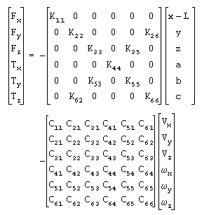
Adams Solver defines each Kij in the following way:
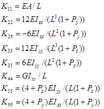
where:
■E = Young’s modulus of elasticity for the beam material.
■A = Uniform area of the beam cross section.
■L = Undeformed length of the beam along the x-axis.
■Py = 12EIzz ASY/(GAL2)
■Pz = 12EIyy ASZ/(GAL2)
■ASY = Correction factor (shear area ratio) for shear deflection in the y direction for Timoshenko beams.
■ASZ = Shear area ratio for shear deflection in the z direction for Timoshenko beams.
Note: | Beams may be also defined to support nonlinear geometric behavior. For details, see the BEAM documentation for Adams Solver (C++). |
Adams Solver applies an equilibrating force and torque at the J marker on the reaction body, as defined by the following equations:
L is the instantaneous displacement vector from the J marker to the I marker. While the force at the J marker is equal and opposite to the force at the I marker, the torque is usually not equal and opposite, because of the force transfer.
Using the Formulation = nonlinear option
When using the Formulation = nonlinear option, then the Euler-Bernoulli formulation is used to define the forces and moments. In this case, Adams uses the following constitutive equations to apply a force and a torque to the I marker.
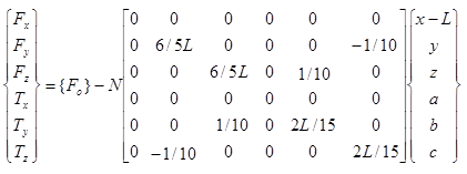
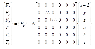
Where {F0} corresponds to the constitutive equations shown above, and N is the axial force on the beam computed as:
N = K11(x - L) + d
The axial force N corresponds to the term Fx computed using linear theory (refer Using the Formulation = linear option). If there is damping (Damping Ratio or Matrix of Damping Terms are defined), the term d corresponds to viscous damping and can be computed as shown above.
The linear theory is the default model for the BEAM statement. The nonlinear theory should be used when the BEAM elements in the model are subject to high axial forces. In those cases, the additional terms in the force/torque equations help stabilize the numerical solution.
Using the Formulation = string option
When using the option Formulation = string, then a simplified Euler-Bernoulli formulation is used to define the forces and moments. In this case, Adams Solver uses the following constitutive equations to apply a force and a torque to the I marker.
Where {F0} and N are computed as described in Using the Formulation = nonlinear option above. This simplification may provide accurate results faster. Notice the stiffness matrices shown in all of the above equations show only a subset of a complete stiffness matrix. The rest of the entries may be found by applying equilibrium conditions.
Creating Beams
To create a beam:
 .
. 2. Select a location for the beam on the first part. This is the action body.
3. Select a location for the beam on the second part. This is the reaction body.
4. Select the direction in the upward (y) direction for the cross-section geometry.
Modifying Beams
After you’ve created a Beam, you can modify the following:
■Markers between which the beam acts.
■Stiffness and damping values.
■Material properties of the beam, such as its length and area.
Learn about Constitutive Equations for Beams.
To modify a beam:
1. Display the Force Modify Element Like Beam dialog box as explained in Accessing Modify Dialog Boxes.
2. In the New Beam Name text box, enter a new name for the beam, if desired.
3. In the Solver ID text box, assign a unique ID number to the beam.
4. Enter any comments about the beam that might help you manage and identify the beam.
5. Enter values for the beam properties as explained in the table below, and then select OK.
To set: | Do the following: |
|---|---|
Area moments of inertia | Enter the following: ■In the Ixx text box, enter the torsional constant. The torsional constant is sometimes referred to as the torsional shape factor or torsional stiffness coefficient. It is expressed as unit length to the fourth power. For a solid circular section, Ixx is identical to the polar moment of inertia J=  . For thin-walled sections, open sections, and non-circular sections, you should consult a handbook. . For thin-walled sections, open sections, and non-circular sections, you should consult a handbook.■In the Iyy and Izz text boxes, enter the area moments of inertia about the neutral axes of the beam cross sectional areas (y-y and z-z). These are sometimes referred to as the second moment of area about a given axis. They are expressed as unit length to the fourth power. For a solid circular section, Iyy=Izz=  . For thin-walled sections, open sections, and non-circular sections, you should consult a handbook. . For thin-walled sections, open sections, and non-circular sections, you should consult a handbook. |
Area of the beam cross section | In the Area of Cross Section text box, enter the uniform area of the beam cross-section geometry. The centroidal axis must be orthogonal to this cross section. |
Shear area ratio | In the Y Shear Area Ratio and Z Shear Area Ratio text boxes, specify the correction factor (the shear area ratio) for shear deflection in the y and z direction for Timoshenko beams. If you want to neglect the deflection due to shear, enter zero in the text boxes. For the y direction: 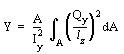 where: ■Qy is the first moment of cross-sectional area to be sheared by a force in the z direction. ■lz is the cross section dimension in the z direction. For the z direction: 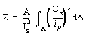 where: ■Qz is the first moment of cross-sectional area to be sheared by a force in the y direction. ■ly is the cross section dimension in the y direction. Common values for shear area ratio based on the type of cross section are: ■Solid rectangular - 6/5 ■Solid circular - 10/9 ■Thin wall hollow circular - 2 Note: The K1 and K2 terms that are used by MSC/NASTRAN for defining the beam properties using PBEAM are the inverse of the y shear and z shear values that Adams View uses. |
Young’s and shear modulus of elasticity | In the Young’s Modulus and Shear Modulus text boxes, enter Young’s and shear modulus of elasticity for the beam material. |
Length of beam | Enter the undeformed length of the beam along the x-axis of the J marker on the reaction body. |
Damping ratio or damping matrix | Select either: ■Damping Ratio and enter a damping value to establish a ratio for calculating the structural damping matrix for the beam. To obtain the damping matrix, Adams Solver multiplies the stiffness matrix by the value you enter for the damping ratio. ■Matrix of Damping Terms and enter a six-by-six structural damping matrix for the beam. Because this matrix is symmetric, you only need to specify one-half of the matrix. The following matrix shows the values to input: 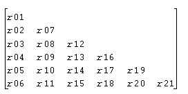 Enter the elements by columns from top to bottom, then from left to right. The damping matrix defaults to a matrix with thirty-six zero entries; that is, r1 through r21 each default to zero. The damping matrix should be positive semidefinite. This ensures that damping does not feed energy into the model. Adams Solver does not warn you if the matrix is not positive semidefinite. |
Markers that define the beam | Specify the two markers between which to define a beam. The I marker is on the action body and the J marker is on the reaction body. The J marker establishes the direction of the force components. By definition, the beam lies along the positive x-axis of the J marker. Therefore, the I marker must have a positive x displacement with respect to the J marker when viewed from the J marker. In its undeformed configuration, the orientation of the I and the J markers must be the same. When the x-axes of the markers defining a beam are not collinear, the beam deflection and, consequently, the force corresponding to this deflection are calculated. To minimize the effect of such misalignments, perform a static equilibrium at the start of the simulation. When the beam element angular deflections are small, the stiffness matrix provides a meaningful description of the beam behavior. When the angular deflections are large, they are not commutative; so the stiffness matrix that produces the translational and rotational force components may not correctly describe the beam behavior. Adams Solver issues a warning message if the beam translational displacements exceed 10 percent of the undeformed length. |
Formulation | Specifies the formulation to be used to define the force and torque this element will apply. By default the liner theory is used (see Using the Formulation = liner option above). If the nonlinear option is used, the full non linear Euler-Bernoulli theory is used. If the string option is used, a simplified non linear theory is used. The simplified non linear theory may speed up your simulations with little performance penalties. |
Field Elements
A field element applies a translational and rotational action-reaction force between two locations. Adams View creates markers at each location. The marker on the first location you specify is called the I marker. The marker on the second location you specify is called the J marker. Adams View applies the component translational and rotational forces for a field to the I marker and imposes reaction forces on the J marker.
The field element can apply either a linear or nonlinear force, depending on the values you specify after you create the field.
■To specify a linear field, enter values that define a six-by-six stiffness matrix, translational and rotational preload values, and a six-by-six damping matrix. The stiffness and damping matrixes must be positive semidefinite, but need not be symmetric. You can also specify a damping ratio instead of specifying a damping matrix.
■To specify a nonlinear field, use the User-written subroutine FIESUB to define the three force components and three torque components and to enter values to pass to FIESUB. (See the Adams Solver Subroutines online help.)
Constitutive Equations for Field Elements
The following constitutive equations define how Adams Solver uses the data for a linear field to apply a force and a torque to the I marker depending on the displacement and velocity of the I marker relative to the J marker.
For a nonlinear field, the following constitutive equations are defined in the FIESUB subroutine:
Adams Solver applies the defined forces and torques at the I marker. In the linear and nonlinear equations:
■Fx, Fy, and Fz are the three translational force measure numbers.
■Tx, Ty, and Tz are the three rotational force measure numbers associated with unit vectors directed along the x-, y-, and z-axes of the J marker.
■K is the stiffness matrix.
■x0, y0, z0, a0, b0, and c0 are the free lengths.
■x, y, z, a, b, and c are the translational and the rotational displacements of the I marker with respect to the J marker expressed in the coordinate system of the J marker.
■Vx, Vy, and Vz are the scalar time derivatives of x, y, and z, respectively.
■x, y, and z are the measure numbers of the angular velocity of the I marker as seen by the J marker, expressed in the J marker coordinate system.
■C is the damping matrix.
■F1, F2, F3, T1, T2, and T3 are the translational and rotational pre-tensions.
Adams Solver computes all variables and time derivatives in the J marker coordinate system.
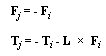
Adams Solver applies an equilibrating force and torque at the J marker, as defined by the following equations:
Fj = - Fi
Tj = - Ti - L Fi
L is the instantaneous displacement vector from the J marker to the I marker. While the force at the J marker is equal and opposite to the force at the I marker, the torque is usually not equal and opposite, because of the force transfer.
Cautions for Field Elements
■For the constitutive equations of a field element to be accurate, at least two of the rotations (a, b, c) must be small. That is, two of the three values must remain smaller than 10 degrees. In addition, if a becomes greater than 90 degrees, b becomes erratic. If b becomes greater than 90 degrees, a becomes erratic. Only c can become greater than 90 degrees without causing convergence problems. For these reasons, it is best to define your field such that angles a and b (not a and c and not b and c) remain small.
■The three rotational displacements (a, b, and c) that define the field are not Euler angles. They are the projected angles of the I marker with respect to the J marker. Adams Solver measures them about the x-, y-, and z-axes of the J marker.
■The K and C matrices must be positive semidefinite. In other words:
xtK x > 0 for all non-zero displacements x, and
ytC y > 0 for all non-zero velocities y
If this is not true, the stiffness matrix of the field may be removing energy from the system. Similarly, the damping matrix may be adding energy to the system. Both of these situations are uncommon. Adams Solver (FORTRAN) does not warn you if the C matrix, K matrix, or both are not positive semidefinite. While Adams Solver (FORTRAN) does not require that these matrices be symmetric, it is most realistic.
Defining the Elements of the Stiffness and Damping Matrices
The elements of the stiffness and damping matrices for a field element have mixed units because each of the 6x6 matrices is assembled from four 3x3 matrices, each having consistent units within itself, but different from each other.
The stiffness matrix is multiplied by displacements (both linear and angular) to give the forces (both linear and torsional). Here (x, y, z) is the displacement vector and (a, b, c) are the displacement angles. F and T are the force and torque vectors.
[ | ] [ x ] [ Fx ]
[ Force/Length | Force/Angle ] [ y ] [ Fy ]
[ | ] [ z ] [ Fz ]
-----------------|--------------- =
[ | ] [ a ] [ Tx ]
[ Torque/Length | Torque/Angle] [ b ] [ Ty ]
[ | ] [ b ] [ Tz ]
Creating Field Elements
When you create a Field element, you define the location of the force element. SD Suspension creates I and J markers defining the location and direction of the field. To define other properties of the field element, such as its damping values, you must modify the field.
To create a field element:
 .
. 2. In the settings container, specify the following:
How you want the force applied to parts. You can select the following:
♦1 Location
♦2 Bodies - 1 Location
♦2 Bodies - 2 Locations
Learn about Applying Multi-Component Forces to Parts.
How you want the force oriented. You can select:
♦Normal to Grid - Lets you orient the force using the x-, y-, and z-axes of the current Working grid, if it is displayed, or using the x-, y, and z-axes of the screen.
♦Pick Feature - Lets you orient the force along a direction vector on a feature in your model, such as the face of a part. The direction vector you select defines the z-axis for the force; Adams View automatically calculates the x- and y-axes.
3. Click the bodies unless Adams View is automatically selecting them.
4. Click one or two force-application points depending on the location method you selected.
5. If you selected to orient the force along a direction vector on a feature, move the cursor around in your model to display an arrow that shows the direction along a feature where you want the force oriented. When the direction vector shows the correct z-axis orientation, click.
Modifying Field Elements
After creating a Field element, you can modify it to define a linear or nonlinear force.
To modify a field element:
1. Display the Force Modify Element Like Field dialog box as explained in Accessing Modify Dialog Boxes.
2. In the New Field Name text box, enter a new name for the field element, if desired.
3. Enter the values in the dialog box as explained the table below, and then select OK.
To set: | Do the following: |
|---|---|
Markers that define the field | In the I marker Name and J marker Name text boxes, specify the two markers between which the force and torque are to be exerted. |
Translational and rotational preload of field | Enter the preload translational and rotational force for the field element in the Preload text boxes. ■Translation at Preload to define three reference lengths. This is the nominal (x0, y0, z0) position of the I marker with respect to the J marker, resolved in the J marker coordinate system. ■Rotation at Preload to define the reference rotational displacement of the axes of the I marker with respect to the J marker, resolved in the J marker axes (a0, b0, and c0) (specified in radians). If the reference force is zero, then the preload is the same as the free length. Entering preload values is optional and defaults to a six zero entry. |
Force preload or parameters to a User-written subroutine | Select one of the following: ■Define Using Standard Values and enter values for the text boxes that appear in the dialog box as explained in the next rows of this table. ■Define Using Subroutine and enter parameters to be passed to the user-written subroutine FIESUB. to define a nonlinear field. Enter up to 30 values (r1[,...,r30]) that Adams View is to pass to FIESUB. For more on the FIESUB subroutine and nonlinear fields, see the Adams Solver online help. You can also specify an alternative library and name for the subroutine in the Routine text box. Learn about specifying your own routine with ROUTINE Argument. |
If you selected Define Using Standard Values, the following options appear: | |
Force and torque preload | In the Force Preload and Torque Preload text boxes, define three preload force components and three preload torque components transferred by the field element when the I and J markers are separated/misaligned by the values specified in the Translation at Preload and Rotation at Preload text boxes. The terms are the force components along the x-, y-, and z-axis of the J marker and the torque components about the x, y-, and z-axis of the J marker, respectively. Entering values for Force Preload and Torque Preload is optional and defaults to six zero entries. |
Stiffness matrix | In the Stiffness Matrix text box, define a six-by-six matrix of stiffness coefficients. The following matrix shows the values to input. 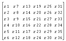 Enter the elements by columns from top to bottom, then from left to right. Learn about Defining the Elements of the Stiffness and Damping Matrices for field elements. Note: A finite element analysis program can give you the values for the stiffness matrix. |
Damping coefficients | Enter either a matrix of damping terms or a damping ratio if you want to include damping coefficients in the calculation of the field forces as explained below. The damping matrix defaults to a matrix with thirty-six zero entries. ■To define a six-by-six matrix of viscous damping coefficients, select Matrix of Damping Terms and enter the elements. The following matrix shows the values to input. Enter the elements by columns from top to bottom, then from left to right. Learn about Defining the Elements of the Stiffness and Damping Matrices for field elements. ■To enter a damping ratio that defines the ratio of the damping matrix to the stiffness matrix, select Damping Ratio and enter the value. If you enter a damping ratio, Adams Solver multiplies the stiffness matrix by the ratio to obtain the damping matrix. Do not enter a ratio without also entering a stiffness matrix. Note: A finite element analysis program can give you the values for the damping matrix. |