About Adjusting Your Model Before Simulation

Before you begin your Simulation, you may want to do one or more preliminary operations to help ensure a better simulation. You can do any of the following:

You can use the Model Verify Tool to check for error conditions in your model, such as misaligned joints, unconstrained parts, or massless parts in dynamic models. The Model Verify tool alerts you to other possible problems. It is a good tool to use periodically as you add detail to or refine your model. The following sections explain how to verify your model and describe more about overconstraining your model.

To learn more about avoiding improper connections, see Performing Initial Conditions Simulation. To manage the mass properties of rigid bodies, see Modifying Mass and Inertia for Rigid Bodies.

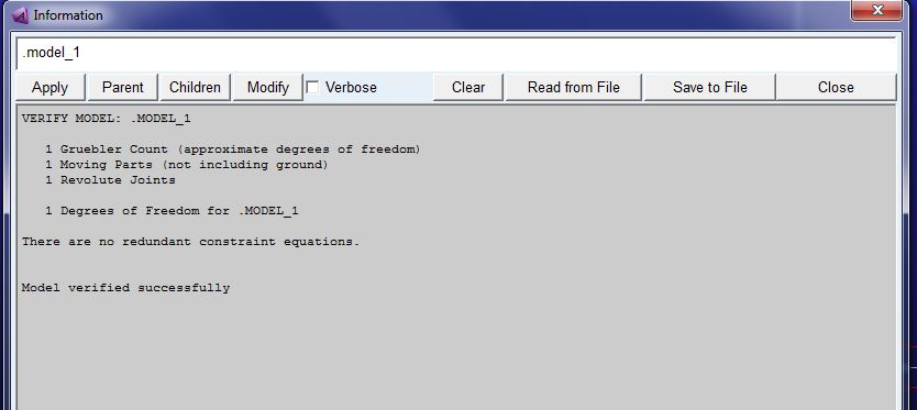
An information window appears with information about your model as shown in the figure below.

Constraints in Adams View remove DOF from your model by adding algebraic constraint equations to the governing system of DAEs (Differential and Algebraic equations). The different constraints in the Adams View constraints library remove different types and number of DOF. Joints can remove anywhere from one to six DOF, depending on their type. For more information on the type and number of DOFs that each joint removes, see Constraints and Degrees of Freedom.

Mathematically, however, Adams Solver represents similarly constrained DOF with similar algebraic equations. The following are representative of the type of algebraic equations Adams Solver uses to represent DOF constrained by joints:

Equation  (1) through Equation  (3) constrain translational DOF, while Equation  (4) through Equation  (6) constrain rotational DOF. The table below explains each of the mathematical equations. In the explanations, the I marker is on the first part and the J marker is on the second part.

The table below lists some of the most commonly used joints and the equations that are used to represent them:

Notice that each of the five joints uses Equations 1 and 2. Duplicating constrained DOF between the same parts can lead to overconstraining your model and introduce redundant constraint equations.

Adams Solver outputs warning messages to help you understand which equations are redundant and, therefore, which DOF are removed more than once. For some examples of warning messages in Adams View and how you can remove the redundancy that they indicate, See Examples of Redundant Constraints Messages.

When building a model, you may find that you define a pair of constraints that constrain two parts in exactly the same way, and so remove identical Degrees of freedom (DOF) from your model. For example, when modeling a door that is connected to a ground-fixed door frame, you might add two hinges (revolute joints) to restrict the door's movement but this is unnecessary. In mathematical terms, the constraint equations of both constraints are redundant with each other because they each remove the same five DOF.

In a physical mechanical system, it might be necessary to have two constraints that restrict the same DOF because of deformation of the parts and joint-play in the connections. In an ideal mathematical model, however, where parts are rigid and joints do not permit any play, only one of the constraints is required and the other constraint is redundant.

Redundant constraints are considered to be either consistent or inconsistent. Redundant constraints are consistent if a solution satisfying the set of independent constraint equations also satisfies the set of dependent or redundant constraint equations. Using the example of the door, the constraints are consistent whenever the axes of the two hinges are aligned. If, however, the axes of the two hinges are not aligned, the door cannot move without breaking one of the hinges. In this case, the two hinges are inconsistent.

When the analysis engine, Adams Solver, encounters redundant constraints, it determines which constraints are redundant, removes them from the set of equations, and provides a set of results that characterizes the motion and forces in the model. In this way, Adams Solver can solve the equations of motion but only if the constraints are consistent. Note that models with redundant constraints do not have a unique solution. Solutions other than the one Adams Solver provides can also be physically realistic.

Redundant constraints that are initially consistent can become inconsistent as your model simulates over time. Adams Solver stops simulating as soon as the redundant constraints become inconsistent. For example, consider a planetary gear system with redundant constraints. Slight misalignment errors can accumulate over time, eventually resulting in a failure of the consistency check. If this occurs, you can remove the redundant constraints or replace them with flexible connections.

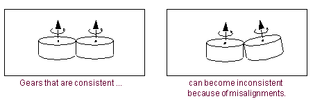
In the case of the door with two hinges, Adams Solver ignores five of the constraint equations that it finds redundant. You do not know which equations Adams Solver ignores, however. If Adams Solver ignores all of the equations corresponding to one of the hinges, then all the reaction forces are concentrated at the other hinge in the Adams Solver solution. Adams Solver arbitrarily sets the reaction forces to zero at the redundant hinge. But Adams Solver might not discard all the equations for one hinge and retain all the equations from the other. It might just as easily retain one or more equations from each, and discard one or more from each.

Although Adams Solver still provides the physically correct solution, the simulation may require extra computational effort to constrain the motion when all of the constraint forces and torques are concentrated at one end of the door. Consequently, it is always a good idea to carefully select your constraints and define models without any redundancies. For example, you can construct the model of the door with a spherical joint and a parallel-axes constraint instead of the single revolute joint.

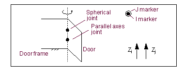
When you verify your model or run a simulation, Adams Solver tells you which constraints are redundant. To solve the redundancy, try replacing a redundant idealized joint with a joint primitive. You may also want to replace redundant constraints with approximately equivalent flexible connections.

Adams Solver does not always check the initial conditions set for a constraint when it performs overconstraint checking. If you apply a motion on one joint and initial conditions on another joint, check to ensure that they are not redundant because Adams Solver does not check them for redundancy and your model may lock up when simulation begins. As a general rule, do not specify more initial conditions than the number of DOF in your model. For more on initial conditions for joints, see Setting Initial Conditions.

The following sections provide examples of redundant constraint messages and ways to avoid the redundancies:

If in your model, Joint_7 is a revolute joint, and Adams View gives you the following warning messages, then you have two redundant constraint equations:

Joint_7 unnecessarily removes Rotation Between Zi and Xj

Joint_7 unnecessarily removes Rotation Between Zi and Yj

These messages indicate that the rotational constraint equations 4 and 5 that the revolute joint introduces are not needed. Therefore, you could replace the revolute joint with a spherical joint since it does not use these equations.

If in your model, Joint_29 is a translational joint, and Adams View displays the following warning messages, then you could change Joint_29 from a translational joint to an inline joint to remove the redundancies:

Joint_29 unnecessarily removes Rotation Between Zi and Xj

Joint_29 unnecessarily removes Rotation Between Zi and Yj

Joint_29 unnecessarily removes Rotation Between Xi and Yj

If you build a fourbar mechanism with four revolute joints, Adams View displays messages similar to the following:

Joint_1 unnecessarily removes Rotation Between Zi and Xj

Joint_1 unnecessarily removes Rotation Between Zi and Yj

Joint_3 unnecessarily removes Rotation Between Zi and Xj

These messages indicate that you could change Joint_1 from a revolute joint to a spherical joint, and change Joint_3 from a revolute joint to a universal or Hooke joint. By changing the joint types, you eliminate the redundant constraint warnings and possibly improve the performance of your solution.

Alternatively, you could also remove the redundancies by changing just one of the revolute joints to an inline joint. There is almost always more than one way to remove redundant constraints. The best way is to select joint types so they match the way your physical system can move. Some of the possible configurations are shown in the figure below.

Remember that Adams Solver does not calculate joint reaction forces in any directions associated with redundant constraint equations because it automatically removes these equations when it performs a simulation. Therefore, you may also want to select your joint types based on where you want to measure joint reaction forces.

The Gruebler count, provides a rough estimate of the number of degrees of freedom (DOF) in the model using the Gruebler equation. In general, the Gruebler count is computed by adding up the number of DOF introduced by parts and subtracting the number of DOF removed by constraints.

Ideally, while computing the Gruebler count for a nonlinear flex body, one should consider all DOF from the finite element mesh defined in the input bulk data file (BDF). However, if we use these DOF in the Gruebler count, the nonlinear flex body DOF will be dominant and the Gruebler count will be too high to reflect the correct/physical DOF of the multibody model. To avoid this issue, Adams Solver converts the nonlinear flex body into an equivalent linear flex body which is used in the Gruebler count computation. It should be noted that the total DOF of this linear flex body are far less than those of the corresponding nonlinear flex body. Thus, the nonlinear flex body DOF do not overshadow the rest of the model's DOF and one gets a better idea of the approximate number of DOF of the entire multibody model.

The DOF for an equivalent linear flex body are computed as:

DOF = number of normal modes + number of constraint modes + 6 (that is, number of rigid-body modes)

When you perform a static equilibrium simulation on your model, Adams Solver iteratively repositions all parts in an attempt to balance all the forces for one particular point in time.

To perform a Static equilibrium simulation, Adams Solver finds the configuration and static forces for which all the static forces in the system balance after being evaluated at the current simulation time. This process requires the solution of a set of nonlinear algebraic equations. Adams Solver uses the modified Newton-Raphson iteration to solve these equations. (To learn more about Newton-Raphson solutions, see the DEBUG statement in the Adams Solver online help.)

If your force and motion inputs change over time and you want to investigate how your equilibrium configurations change, you can choose to perform a series of static simulations over an interval of time. A series of static simulations is often referred to as a quasi-static simulation because time is allowed to vary between static simulations but time-varying inertial effects are neglected for each individual static simulation. Quasi-static simulations are useful for approximating the dynamic response of models that move very slowly and for which you can assume that the effects of inertial force can be neglected.

Since Adams Solver must be able to move parts around as it attempts to iterate to an equilibrium configuration, it does not make sense to perform a static simulation on a model that has no degrees of freedom (DOF). If the model has no DOF, no parts are allowed to move.

When you select to perform a Dynamic simulation to find the Static equilibrium, Adams Solver performs a standard dynamic simulation, except for the following:

Because a dynamic simulation occurs, the settings in Solver Settings - Dynamics specify the error tolerances and other parameters normally associated with dynamic simulations.

You can perform an Initial conditions simulation to check for any inconsistencies in your model. The initial conditions simulation is often referred to as an assemble model operation. An initial conditions simulation tries to reconcile any positioning inconsistencies that exist in your model at its design configuration and make it suitable for performing a nonlinear or Linear simulation. Most importantly, the initial conditions simulation tries to ensure that all joint connections are defined properly.

For example, for a revolute joint to be defined properly, the origins of the markers that define the joint must be coincident throughout a simulation. If the markers are not coincident, the joint is broken and needs to be repaired. In this example, the initial conditions simulation helps repair the broken revolute joint by moving the origins of the two markers until they are coincident, as shown in the following figure.

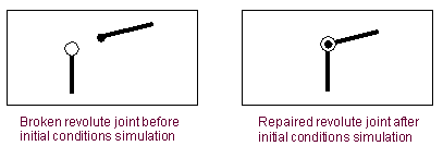
You can also use the initial conditions simulation if you are creating parts in exploded view. Exploded view is simply creating the individual parts separately and then assembling them together into a model. You might find this convenient if you have several complicated parts that you want to create individually without seeing how they work together until much later. Adams View provides options for specifying that you are creating your model in exploded view as you create constraints.