Run-Time Functions Categories
The two major types of run-time functions are:
System-Supplied Run-Time Functions
This section introduces you to the run-time functions categories as they appear in the Function Builder. For more details regarding each function, please see Run-Time Functions Examples.
Note that although some run-time functions have the same names as certain design-time functions, they only work with a model at an analysis-time step.
The following sections give you an overview of the run-time functions categories. The functions categories are presented in the order they appear in the Function Builder.
1. Displacement Functions
Displacement functions return scalar measures associated with a particular component of the translational displacement vector from one coordinate system marker to another or an angular displacement from one coordinate system marker to another.
You can use the displacement functions during a simulation to obtain from Adams the displacement measurements of an object. Displacement functions provide measurements that can be useful in:
■Plotting displacement measurements.
■Creating equations which depend on the displacement of an object.
■Monitoring the displacement of an object and triggering the occurrence of special events when the displacement reaches a certain value.
The following table lists the names and definitions for the displacement functions:
This function: | Returns: |
|---|---|
An x component of the translational displacement vector from one coordinate system marker to another. | |
A y component of the translational displacement vector from one coordinate system marker to another. | |
A z component of the translational displacement vector from one coordinate system marker to another. | |
The magnitude of the translational displacement vector from one coordinate system marker to another. | |
The rotational displacement (in radians) of one coordinate system marker about the x-axis of another. | |
The rotational displacement (in radians) of one coordinate system marker about the y-axis of another. | |
The rotational displacement (in radians) of one coordinate system marker about the z-axis of another. | |
The first angle of rotation (in radians) associated with a body-fixed 321 rotation sequence from one coordinate system marker to another. | |
The negative of the second angle of rotation (in radians) associated with a body-fixed 321 rotation sequence from one coordinate system marker to another. | |
The third angle of rotation (in radians) associated with a body-fixed 321 rotation sequence from one coordinate system marker to another. | |
The first angle of rotation (in radians) associated with a body-fixed 313 rotation sequence from one coordinate system marker to another. | |
The second angle of rotation (in radians) associated with a body-fixed 313 rotation sequence from one coordinate system marker to another. | |
The third angle of rotation (in radians) associated with a body-fixed 313 rotation sequence from one coordinate system marker to another. |
2. Velocity Functions
Velocity functions return a requested magnitude or component of the translational or rotational velocity vector between two markers.
You can use the velocity functions during a simulation to obtain from Adams the velocity measurements of an object. Velocity functions provide measurements that can be useful in:
■Plotting velocity measurements.
■Creating equations that depend on the velocity of an object.
■Monitoring the velocity of an object and triggering the occurrence of special events when the velocity reaches a certain value.
The following table lists the names and definitions for the velocity functions:
Function: | Returns: |
|---|---|
An x component of the difference between the velocity vectors of two coordinate system markers. | |
A y component of the difference between the velocity vectors of two coordinate system markers. | |
A z component of the difference between the velocity vectors of two coordinate system markers. | |
The magnitude of the first time-derivative of the displacement vector between two coordinate system markers. | |
An x component of the difference between the angular velocity vectors of two coordinate system markers. | |
A y component of the difference between the angular velocity vectors of two coordinate system markers. | |
A z component of the difference between the angular velocity vectors of two coordinate system markers. | |
The magnitude of the difference between the angular velocity vectors of two coordinate system markers. | |
The radial (relative) velocity to one coordinate system marker from another. |
3. Acceleration Functions
Acceleration functions return a requested magnitude or component of the translational or rotational acceleration vector between two markers.
You can use the acceleration functions during a simulation to obtain from Adams the acceleration measurements of an object. Acceleration functions provide measurements that can be useful in:
■Plotting acceleration measurements.
■Creating equations that depend on the acceleration of an object.
■Monitoring the acceleration of an object and triggering the occurrence of special events when the acceleration reaches a certain value.
The WDT prefix used for angular acceleration functions implies  or omega-dot, the time derivative of angular velocity.
or omega-dot, the time derivative of angular velocity. The following table lists the names and definitions for the acceleration functions:
Function: | Returns: |
|---|---|
An x component of the difference between the acceleration vectors of two coordinate system markers. | |
A y component of the difference between the acceleration vectors of two coordinate system markers. | |
A z component of the difference between the acceleration vectors of two coordinate system markers. | |
The magnitude of the second time-derivative of the displacement vector to one coordinate system marker from another coordinate system marker. | |
An x component of the difference between the angular acceleration vectors of two coordinate system markers. | |
A y component of the difference between the angular acceleration vectors of two coordinate system markers. | |
A z component of the difference between the angular acceleration vectors of two coordinate system markers. | |
The magnitude of the difference between the angular acceleration vectors of two coordinate system markers. |
4. Contact Functions
You can use contact functions to define collision forces. The functions are built so as to turn on and off during simulation, which makes them useful for representing bodies that come into intermittent contact with one another.
The following table lists the names and definitions for the contact functions:
Function: | Returns: |
|---|---|
A real number for a force magnitude corresponding to a one-sided collision, using a compression-only nonlinear spring-damper formulation. | |
A real number for a force magnitude corresponding to a two-sided collision, using a compression-only nonlinear spring-damper formulation. |
5. Spline Functions
Splining is a method of interpolation that allows derivation of intermediate locations on a curve or surface between known points.
You can use spline functions during a simulation to define smooth functions to approximately fit data points. Spline functions can be useful when:
■Driving a motion with test data.
■Defining a force with test data.
■Plotting smooth curves through data points.
The following sections provide more information about splines:
Interpolation Methods Overview
Adams View allows you to use three interpolation methods, as shown below:
Interpolation methods: | Fit characteristic: | Function name: | Advantages: | Disadvantages: |
|---|---|---|---|---|
Cubic spline | Global | CUBSPL | ■Accurate derivatives ■Curve ■Surface | ■Not as fast ■Some waviness |
B-spline | Global | CURVE | ■Accurate derivatives ■Can be user-defined with CURSUB | Curve only (no surface) |
Akima | Local | AKISPL | ■Fast ■Curve ■Surface | Inaccurate derivatives |
Comparison of Interpolation Methods
The Akima interpolation is a local fit. Local methods require information only about points in the vicinity of the interval being interpolated to define the coefficients of the cubic polynomial. This means that each data point in an Akima spline only affects the nearby portion of the curve. Since it uses local methods, Akima is very fast.
Akima always produces good results for the value of the function being approximated. AKISPL returns good estimates for the first derivative of the approximated function when the data points are evenly spaced. In instances where the data points are unevenly spaced, the estimate of the first derivative may be in error. In all cases, the second derivative of the function being approximated is unreliable.
The cubic interpolation is a global fit. Global methods use all the given points to calculate all the coefficients for all the intervals in question, simultaneously. Therefore, each data point affects the entire cubic spline: if you move one point the whole curve changes accordingly, making a cubic spline wigglier and harder to force into a desired shape. This is especially noticeable on functions with linear portions or sharp changes in the curve. In these cases, a cubic spline will almost always have more wiggles than an Akima spline.
Both global and local methods work well on smoothly-curving functions.
CUBSPL, though not as fast as AKISPL, always produces good results for the value of the function being approximated, as well as its first and second derivatives. The data points don't have to be evenly spaced. The solution process often requires estimates of derivatives of the functions being defined. The smoother a derivative is, the easier it is for the solution process to converge.
Smooth (continuous) second derivatives are important if you use the spline in a motion. The second derivative is the acceleration enforced by the motion, which defines the reaction force required to drive the motion. A discontinuity in the second derivative means a discontinuity in the acceleration and therefore in the reaction force. This can cause poor solver performance or even failure to converge at the point of discontinuity.
The B-spline interpolation method is primarily designed to describe 3D geometric curves. Although the B-spline can be useful for geometric applications, you should use AKISPL or CUBSPL to construct most motions, forces, and other such entities.
Where to Find the Spline Functions
The following table lists the names and definitions for the spline functions:
Function: | Returns: |
|---|---|
Either a derivative of a curve or an interpolated value from a curve or surface. | |
A B-spline or a user-written curve created by a CURVE data element. | |
Either a derivative of a curve or an interpolated value from a curve or surface. | |
Derivative of the interpolated value of a spline. |
6. Force in Object Functions
Force in object functions are used to return instantaneous force values generated by modeling elements.
The following sections further explain the force in object functions:
Using the Force in Object Functions
You can use the force in object functions during a simulation to obtain from Adams the force measurements due to constraints (such as joints and motions), compliant connections (such as spring-dampers and bushings), and applied forces (such as multiple-component general-equation force elements). The force in object functions provide measurements that can be useful in:
■Plotting the force measurements.
■Creating equations for other forces whose magnitudes depend on these forces.
■Monitoring force magnitudes and triggering the occurrence of special events when these forces reach certain values.
Constraint Characteristics
Most constraints have the following characteristics:
■Connect two bodies, referred to as the first body and second body or the action and reaction body respectively.
■Are applied at two distinct points, though sometimes coincident.
■Depend on coordinate system axes to define constraint direction.
■Apply whatever forces are required to prevent movement in certain directions.
■Do not require the user to define the magnitudes of the forces they apply since Adams automatically calculates force magnitudes.
Force Characteristics
Most forces have the following characteristics:
■Are applied to two bodies, referred to as the first body and second body.
■Are applied at two distinct points, though sometimes coincident.
■Depend on coordinate system axes to define force application.
■Require the user to define the magnitudes of the forces they apply.
In Adams, you can define force magnitudes in two ways:
1. With linear spring-damper-like elements that use predefined equations that automatically depend only on displacement and velocity directly; for these forces you can simply input stiffness and damping coefficients.
2. With multiple-component, general-equation force elements that have no predefined equations. These allow you to create your own force magnitude equations with no restrictions on the dependencies.
When you define your own equations for force magnitudes, you have to tell Adams what the force depends on. For instance, a force could depend on the displacement between two coordinate system markers or their relative velocity or acceleration, or the force applied to a coordinate system marker by a constraint or force element.To help you define these dependencies, Adams offers you displacement functions (Displacement Functions), velocity functions (Velocity Functions), acceleration functions (Acceleration Functions), resultant force functions (Resultant Force Functions), as well as force in object functions.
Whenever you use the force in object functions, you must tell Adams how you want the force to be measured. You must specify:
■Which force-applying object you want to measure. For example: joint_4, motion_6, sforce_3, gforce_19, and so on.
■On which body you want to take the measurement, the first body or the second body.
■Which force vector component you want to obtain.
Using a Force in Object Function
In this example we'll calculate the force acting on a block located on an incline, as illustrated in body 1. Before working through this example, reference Six-component Force/Torque (GFORCE).
This example consists of a system defined as follows:
■A translational joint (JOINT_1) connects a block and an incline by way of coordinate system markers named block.marker_14 and incline.marker_15.
■A fixed joint (JOINT_2) connects the incline to ground by way of incline.marker_32 and ground.marker_33.
■A general-equation, multiple-component force, named GForce_7 is applied to the block, normal to the surface of the incline.
■The GForce_7 is applied to block.marker_28 and ground.marker_29, so that the block is the action body and ground is the reaction body.
■There is no gravity.
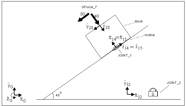
In this example, GFORCE is defined as: 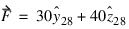 .
.
. The GFORCE yields different results, as we change the arguments used:
GFORCE(GForce_7, 0, 2, block.marker_28) = 0
GFORCE(GForce_7, 0, 3, block.marker_28) = 30
GFORCE(GForce_7, 0, 4, block.marker_28) = 40
GFORCE(GForce_7, 0, 1, block.marker_14) = 50
GFORCE(GForce_7, 0, 2, block.marker_14) = - 40
GFORCE(GForce_7, 0, 3, block.marker_14) = 0
GFORCE(GForce_7, 0, 4, block.marker_14) = - 30
GFORCE(GForce_7, 1, 1, block.marker_28) = 50
GFORCE(GForce_7, 1, 2, block.marker_28) = 0
GFORCE(GForce_7, 1, 3, block.marker_28) = - 30
GFORCE(GForce_7, 1, 4, block.marker_28) = - 40
Where to Find the Force in Object Functions
The following table lists the names and definitions for the force in object functions:
Function: | Returns: |
|---|---|
A force or torque induced by a specified joint on one of the two bodies connected by the joint object. | |
A force or torque component induced by a specified motion on one of the two bodies affected by the motion object. | |
A force or torque induced by a specified point-to-curve object on one of the two bodies connected by the point-to-curve object. | |
A force or torque induced by a specified curve-to-curve object on one of the two bodies connected by the curve-to-curve object. | |
A force or torque induced by a specified joint primitive on one of the two bodies connected by the joint primitive. | |
A force or torque applied by a specified single-component force on one or two bodies directly affected by the single-component force. | |
A force or torque applied by a specified three-component force on one or two bodies directly affected by the three-component force. | |
A force or torque applied by a specified three-component torque on one or two bodies directly affected by the three-component torque. | |
A force or torque applied by a specified six-component force/torque on one or two bodies directly affected by the six-component force / torque. | |
A force or torque applied by a specified multipoint force on one or two bodies directly affected by the multipoint force. | |
A force or torque applied by a specified beam force on one or two bodies directly affected by the beam force. | |
A force or torque applied by a specified bushing force on one or two bodies directly affected by the bushing force. | |
A force or torque applied by a specified field force on one or two bodies directly affected by the field force. | |
A force or torque applied by a specified spring-damper force on one or two bodies affected by the spring-damper force. |
7. Resultant Force Functions
Resultant force functions return either the net applied action and reaction force between two markers, or the net applied action-only forces at a marker.
Where to Find the Resultant Force Functions
The following table lists the names and definitions for the resultant force functions:
Function: | Returns: |
|---|---|
An x component of the net translational force acting at one coordinate system marker due to all applied forces and constraints acting between that coordinate system marker and another. | |
A y component of the net translational force acting at one coordinate system marker due to all applied forces and constraints acting between that coordinate system marker and another. | |
A z component of the net translational force acting at one coordinate system marker due to all applied forces and constraints acting between that coordinate system marker and another. | |
The magnitude of the net translational force acting at one coordinate system marker due to all applied forces and constraints acting between that coordinate system marker and another. | |
An x component of the net torque acting at one coordinate system marker due to all applied torques and constraints acting between that coordinate system marker and another. | |
A y component of the net torque acting at one coordinate system marker due to all applied torques and constraints acting between that coordinate system marker and another. | |
A z component of the net torque acting at one coordinate system marker due to all applied torques and constraints acting between that coordinate system marker and another. | |
The magnitude of the net torque acting at one coordinate system marker due to all applied torques and constraints acting between that coordinate system marker and another. |
8. Math Functions
Math functions apply to scalar numbers or matrices. If you input a scalar, Adams returns a scalar. If you input a matrix, Adams returns a matrix.
Where to Find the Math Functions
The following table lists the names and definitions for the math functions:
Function: | Does the following: |
|---|---|
Returns the absolute value of an expression that represents a numerical value. | |
Returns the arc cosine of an expression that represents a numerical value. | |
Returns the nearest integer whose magnitude is not larger than the integer value of a specified expression that represents a numerical value. | |
Returns the nearest integer whose magnitude is not larger than the real value of an expression that represents a numerical value. | |
Returns the arc sine of an expression that represents a numerical value. | |
Returns the arc tangent of an expression that represents a numerical value. | |
Returns the arc tangent of two expressions each representing a numerical value. | |
Evaluates a Chebyshev polynomial at a user-specified numerical value. | |
Returns the cosine of an expression that represents a numerical value. | |
Returns the hyperbolic cosine of an expression that represents a numerical value. | |
Returns the positive difference of the instantaneous values of two expressions, each representing a numerical value. | |
Returns the value ex, where x is any expression that represents a numerical value. | |
Evaluates a Fourier Cosine series at a user-specified value x. | |
Evaluates a Fourier Sine series at a user-specified value x. | |
Defines a haversine function. HAVSIN is most often used to represent a smooth transition between two functions. | |
Regenerates a time signal from a power spectral density description. | |
Returns the natural logarithm of an expression that represents a numerical value. | |
Returns log to base 10 of an expression that represents a numerical value. | |
Returns the maximum of two expressions that represent numerical values. | |
Returns the minimum of two expressions that represent numerical values. | |
Returns the remainder when one expression representing a numerical value is divided by another expression that represents a numerical value. | |
Evaluates a standard polynomial at a user-specified value x. | |
Transfers the sign of one expression representing a numerical value to the magnitude of another expression representing a numerical value. | |
Evaluates a simple harmonic function. | |
Returns the sine of an expression that represents a numerical value. | |
Returns the hyperbolic sine of an expression that represents a numerical value. | |
Returns the square root of an expression that represents a numerical value. | |
Approximates the Heaviside step function with a cubic polynomial. | |
Provides approximations to the Heaviside step function with a quintic polynomial. | |
Returns a constant amplitude sinusoidal function with linearly increasing frequency. | |
Returns the tangent of an expression that represents a numerical value. | |
Returns the hyperbolic tangent of an expression that represents a numerical value. |
9. Vector Functions
Vector functions represent the class of functions that carry out vector operations. The following table lists the names and definitions for the Vector functions available through the Function Builder:
Function: | Returns: |
|---|---|
A translational displacement vector between two coordinate system markers. | |
A unit vector in the X-axis direction of a coordinate system marker resolved in the coordinate system of another marker | |
A unit vector in the Y-axis direction of a coordinate system marker resolved in the coordinate system of another marker | |
A unit vector in the Z-axis direction of a coordinate system marker resolved in the coordinate system of another marker | |
Difference between the acceleration vectors of two coordinate system markers resolved in the coordinate system of another marker | |
The net translational force vector acting on a coordinate system marker expressed in the coordinate system of another marker | |
The net translational torque vector acting on a coordinate system marker expressed in the coordinate system of another marker | |
Difference between the velocity vectors of two coordinate system markers resolved in the coordinate system of another marker | |
Difference between the angular velocity vectors of two coordinate system markers resolved in the coordinate system of another marker | |
Difference between the angular acceleration vectors of two coordinate system markers resolved in the coordinate system of another marker | |
The unit vector in the direction of an arbitrary vector expression | |
The transformed vector of an arbitrary vector expression resolved between two coordinate system markers |
10. Data Element Access
Data elements give you access to the values of states of generic system modeling entities.
Where to Find Data Elements
The following table lists the names and definitions for the data elements available through the Function Builder:
Function: | Returns: |
|---|---|
The current value of the variable defined by the specified state variable modeling entity. | |
The value of the specified element of the specified array modeling entity. | |
The integrated value of the variable defined by the specified differential equation modeling entity. | |
The value of the variable defined by the specified differential equation modeling entity. | |
The run-time value of a plant input. | |
The run-time value of a plant output. | |
The run-time scored value of a sensor. | |
The run-time value of a contact data. |
11. User-Written Subroutine Invocation
The user-written subroutine invocation allows for values to be passed into subroutines that you create in order to define enhanced function expressions. Only certain modeling elements allow you to define them by way of your own customized subroutines. For more information about subroutines, see the guide, Using Adams Solver Subroutines.
Where to Find the User-Written Subroutine
The following table lists the name and definition for the user-written subroutine.
Function: | Does the following: |
|---|---|
Passes one or more values that are used as parameters in a user-written subroutine. |
12. Constants & Variables
Constants and variables represent values that are frequently used to perform mechanical system simulation, such as time or conversion functions between angular units of radians and degrees.
Where to Find Constants and Variables
The following table lists the names and definitions for the constants and variables:
Function: | Returns: |
|---|---|
The ratio of the circumference of a circle to its diameter (  ). ). | |
The radians-to-degree units conversion factor (180/  ). ). | |
The degrees-to-radian units conversion factor (  /180). /180). | |
The current simulation time. | |
An integer value indicating the current analysis mode. |
User-Supplied Run-Time Functions
User-supplied run-time functions are parameterized runtime functions that are defined by the user that contain an expression which is made up of a combination of design variables, system supplied functions, design time expressions and constants.
User-supplied run-time functions consist of an expression whose evaluated form will be used by the solver at the time of simulation.
You can create these functions via Adams View command language, using the "runtime_function create" command. Alternatively, you can create them using the Function Builder in runtime mode. During creation you must specify the text of the run-time function and optionally the parameter names. When you use these functions, Adams substitutes the user parameters (if any) into the function text in place of the parameter names.
For example:
runtime_function create &
runtime_function_name = runtime_func__1 &
text_of_expression = "-1.0*(DM(P1, P2)-400.0)-0.001*VR(P1, P2)" &
argument_names = "P1", "P2" &
In the example above, P1 and P2 are the formal arguments to the function runtime_func__1.
We can apply above function on sforce.
For Example:
force modify direct single_component_force &
single_component_force_name = .MODEL_1.SFORCE_1 &
function = "runtime_func__1(.MODEL_1.PART_2.MARKER_1, .MODEL_1.PART_2.MARKER_2)"
One can also use an Adams ID instead of the full object name.
For Example:
force modify direct single_component_force &
single_component_force_name = .MODEL_1.SFORCE_1 &
function = "runtime_func__1(1,2)"
Expanded form
Adams expands the expression by replacing the arguments for the formal parameters before exporting to an Adams Solver dataset (.adm file) or passing to Adams Solver from Adams View.
For Example:
Exporting an .adm file, the above runtime_func__1 applied to sforce_1 will be expand like so in the .adm file:
FUNCTION = -1.0*(DM(1, 2)-400.0)-0.001*VR(1, 2)
Therefore, like other forms of design-time model parameterization, the parametrized version of the expression can only be found in the Adams View representation of the model.
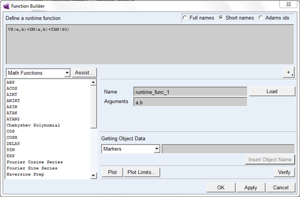
UI
You can create user-written run-time functions using the function builder. The function builder launched from two ways:
1. Main menu:
Tools → Function Builder → Runtime Mode
2. Ribbon based menu:
Ribbon menu → Elements Tab → Function container → Click  icon
icon
Function Builder for run-time functions
User-written run-time function in model browser
After creating run-time function, you can view it Model browser:
Elements → Functions