Running Full-Vehicle Analyses
You can take previously created suspension subsystems and integrate them with other subsystems to create a full-vehicle assembly. You can then perform various analyses on the vehicle to test the design of the different subsystems and see how they influence the total vehicle dynamics. All of the analyses, except for the data-driven analyses, use the .__MDI_SDI_TESTRIG, and are therefore based on the Driving Machine. You can also examine the influence of component modifications, including changes in spring rates, damper rates, bushing rates, and anti-rollbar rates, on the total vehicle dynamics.
Each type of analysis you perform requires a minimum set of subsystems: front and rear suspension subsystems, front and rear wheel subsystems, one steering subsystem, and one body subsystem. Before you can create an assembly and perform an analysis in Adams Car, you must open or create the minimum set of subsystems required.
Using Adams Car, you can:
■Easily modify the geometry and the properties of the components of your subsystems.
■Select from a standard set of vehicle maneuvers to evaluate handling characteristics of your virtual prototype.
■View the vehicle states and other characteristics through plots.
You can specify inputs to the analysis by typing them into an analysis dialog box or by selecting a driver control file that contains the desired inputs.
After specifying the prototype assembly and its analysis, Adams Car, like your company's testing department, applies the inputs that you specified and records the results. To understand how your prototype behaved during the analysis, you can plot the results. After viewing the results, you might modify the prototype and analyze it again to see if your modifications improve its behavior.
The following figure shows an overview of the full-vehicle analysis process.
Setting up Full-Vehicle Analyses
Before you set up a full-vehicle analysis, you must assemble and check the vehicle, as explained next:
Assembling a Vehicle
Adams Car creates a full-vehicle assembly from a set of subsystems that you select. An assembly lets you quickly put together full vehicles from previously tested and verified subsystems and switch between subsystems depending on the analysis that you want to perform.
The associated component property files, such as springs and bushings, must also exist in your database.
If a suspension subsystem uses mount parts, such as the spring top mounting to a subframe, you must read the subframe subsystem into the assembly. If you do not read in the required mount subsystems, Adams Car connects any mount parts to the global ground part instead of the absent mount subsystem. Therefore, the mount point cannot move with the full vehicle, which causes the Adams Car analysis to fail.
Checking a Vehicle
Before submitting your model for analysis, visually check its assembly. The Adams Car default view is front isometric view. From the front view, you should be able to see obvious assembly problems. You should also check your vehicle from the side because it provides a more useful view for positioning the subsystems.
As you view your assembly from different angles, check for obvious problems, such as:
■Is the front suspension in the correct place?
■Is the body graphic positioned correctly?
■Are the wheels somewhere near the same height?
All the analyses currently available are based on the Driving Machine. Therefore, to perform open-loop, closed-loop, and quasi-static analyses, you must select the .__MDI_SDI_TESTRIG in your assemblies. Always check whether you selected the correct test rig for the analysis you want to perform. If you selected an incorrect test rig, create another assembly using the correct test rig.
To check the test rig:
1. From the File menu, point to Info, and then select Assembly.
2. In the Assembly Name text box, enter the name of your assembly.
3. Select OK.
Adams Car displays the Information window, with the test rig name listed at the top of the window.
Setting up the Analysis
Before you submit the full vehicle analysis, you can refer to Vehicle Set-Up utilities. Adams Driver makes use of parameters like Rack Ratio & Steering Ratio when executing the full vehicle simulations.
For example, when the tierod is positioned in front of wheel center, then you need to negate the Rack Ratio value or vice versa for proper motion transfer from rack to wheels, so the vehicle steers as desired.
To set the Rack ratio and other full vehicle parameters, go to Simulate → Full-Vehicle Analysis → Vehicle Set-Up → Set Full Vehicle Parameters.
You have an option to set the desired static vehicle parameters like wheel alignment, corner loads, ride height and wheel rates. To achieve desired vehicle set-up, go to Simulate → Full-Vehicle Analysis → Vehicle Set-Up → Static Vehicle set up. The Static Vehicle Set-Up analysis lets you set desired alignment values for suspension, corner-weights, ride height and wheel rate adjustments at static equilibrium condition.
To plot the results from static and dynamic steps please refer Duplicate Points from PPT Preferences - Plot to handle the duplicate time values on a curve.
To set different road profile for each individual tire, like for example if you want to run the left side wheels over a bump and right-side wheels on flat road, go to Simulate → Full-Vehicle Analysis → Vehicle Set-Up → Set Road for Individual Tires.
Additional vehicle set-up utilities are available such as Set Powertrain Parameters and Set SDI Request Activity.
To set up full-vehicle analyses:
1. From the Simulate menu, point to Full-Vehicle Analysis, and then select the analysis you want to set up.
2. Enter the parameters needed to control the analysis.
3. Typically, each transient analysis can be preceded by a quasi-static prephase analysis before running the transient analysis on your full-vehicle assemblies. A quasi-static prephase analysis consists of a straight analysis or a skidpad analysis, depending on the type of analysis you selected. If you do not select the quasi-static option, Adams Car performs a SETTLE analysis.
For more information about the different quasi-static setup method keywords (such as SETTLE and STRAIGHT), see Structure of Event Files.
4. For dialog box help, select F1.
5. Select OK.
Controlling Full-Vehicle Analyses
If you are an experienced Adams Car user and you want to perform some non-standard full-vehicle analyses, such as studying the linear behavior of your vehicle between two mini-maneuvers, you can use an Adams Solver control subroutine (Eventxxx) to do so.
When you run a full-vehicle analysis, Adams Car writes a number of files to the current working directory (as defined by File -> Select Directory). These files contain important information about the details of the maneuver. In particular, two files are important in defining the scope of the maneuver. These are the Adams Solver control file (.acf) and the event file (.xml). See Working with Event Files (.xml).
The following shows the typical contents of an .acf:
file/model=test_step
preferences/solver=F77
output/nosep
control/ routine=abgVDM::EventInit, function=user(3,1,10,0,2,5,7,17)
control/ routine=abgVDM::EventRunAll, function=user(0)
!
stop
In the .acf, note the following line:
control/ routine=abgVDM::EventInit, function=user(3,1,10,0,2,5,7,17)
This line calls an Adams Car-specific control subroutine (a consub). The consub sets up and initializes the full-vehicle analysis. It does the following:
■Reads the event file (or converts the TeimOrbit .dcf file into XML)
■Performs a number of static analyses based on the content of the DcfStatic class in the event file
■Performs a dynamic analysis by running each of the mini-maneuvers listed in the DcfMini classes in the event file
You can view and modify the event file (.xml) using the Event Builder. The Event Builder allows you to modify existing parameters for the entire maneuver, such as step size and hmax, to modify specific mini-maneuver information, and add mini-maneuvers.
The following line calls the control subroutine EventInit:
control/ routine=abgVDM::EventInit, function=user(3,1,10,0,2,5,7,17)
The call to this subroutine passes 8 parameters, as described next. Note that each number in the array (3,1,10,0,2,5,5,17) is listed after the description of that parameter.
par(1) 3: ID of STRING statement containing .XML event filename = 3
par(2) ID of ORIGO marker = 1
par(3) ID of ARRAY statement containing initial condition SDI parameters = 10
par(4) ID of ARRAY statement containing ids of parts for which initial velocity are not set = 0
par(5) ID of ARRAY holding Vehicle Parameters. = 2
par(6) ID of main Driving Machine ARRAY. = 5
par(7) ID ISO EAS Marker = 7
par(8) ID of ARRAY containing the ids of extensible end condition sensor elements = 17
If you look at the corresponding Adams Solver dataset (.adm), you will see that STRING/3 contains the name of the event file:
! adams_view_name='testrig_dcf_filename'
STRING/3
, STRING =example_crc.xml
All standard Adams Car events generate an event file in XML format, similar to the one referenced in the example above, but .dcf files in TeimOrbit format are still supported, both in the Event Builder and at the solver level. This means that you can replace the above string and reference a .dcf file in TeimOrbit format. The file will be automatically converted to XML format.
By modifying the .acf file, you can now execute all mini-maneuvers defined in the event file, or just run the initialization and then execute one mini-maneuver at a time. Full-vehicle analysis .acf files by default call the Driving Machine initialization routine, then call the RunAll method. You can, however, modify the .acf file and use the following commands for more control over your analysis:
■control/ routine=abgVDM::EventRunAll, function=user(0) - Runs all the active mini-maneuvers in the list of events
■control/ routine=abgVDM::EventRunNext, function=user(0) - Runs the following mini-maneuver in the list of the events
■control/ routine=abgVDM::EventRunFor, function=user(double time) - Runs the current mini-maneuver for duration of time [s]
■control/ routine=abgVDM::EventRunUntil, function=user(double time) - Runs the current mini-maneuver until the desired absolute time [s]
Using this flexibility within the event control subroutine enables you to use the power of the acf language to make changes and re-submit your solution to Adams Solver. The language parameters for the .acf file are documented in the Adams Solver online help.
Running with External Adams Solver
How you run Adams Solver depends on the platform you are on:
■On Windows - The location of your .acf, .adm, and event files is important. Open a DOS shell (from the Start menu, point to Programs, point to Accessories, and then select Command Prompt) and change directory to the location where your files are stored (cd temp\run).
■On Linux - Open a shell and change directory to the location of your files (cd /usr/home/user/temp/run).
To run external Adams Solver:
■Issue the command:
adamsxx acar ru-solver filename.acf
where:
■xx corresponds to the version of Adams that you are using
■filename.acf is the name of your acf file
Reading Results
After you run the analysis, you can use Adams PostProcessor to animate and view the results.
Notes: | ■To control the execution of the various mini-maneuvers defined in the XML event file you need to issue the EventInit control subroutine command first. This instructs Adams Car to build a list of quasi-static and transient events as they are defined in the event file. ■To execute each mini-maneuver in the event file, you should issue a control/ routine=abgVDM::EventRunNext as described above. |
Durability Events
Dynamic Loadcase
A dynamic loadcase analysis actuates the assembly at the wheel center via user defined runtime function expressions or by referencing channel number from RPC3 file. You can do two types of analysis, force based and displacement based.
For Force based analysis (Jack Excitation mode = Force), the gforce at the wheel centres are used to actuate wheel part (spindle) of the assembly.
For displacement-based analysis (jack excitation mode set to Displacement, Velocity and Acceleration), the motions are used to actuate wheels of assembly through jack (dummy parts).
For steering input, it is also possible to define a runtime function expression or by referencing channel number from RPC3 file for the steering motion, thereby combining vertical excitation with steering sweeps.
The controller gains (stiffness and damping) and feedback channel used as inputs to the feed-forward controller system, which is used for force based input analysis.
To set up a Dynamic Loadcase analysis:
1. From the Simulate menu, point to Full-Vehicle Analysis, point to Durability Events, and then select Dynamic Loadcase.
2. Enter the necessary parameters as explained in the dialog box help for Full-Vehicle Analysis: Dynamic Loadcase.
3. Select OK.
Event Set and Event Browser
Event UDE
The event UDE is the user-defined element stored in the database that provides access to the event objects which are displayed in the event browser. All event sets are stored in the special library: .EVENT_SETS. The event UDE stores this information for the definition of the event:
■Assembly reference - model to be used for the analysis
■Variant reference - variant to the used for the analysis
■Event set - Event set parent which stores the event
■Macro reference - This is an object reference to the event type that the event should use for the analysis
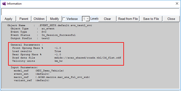
In addition to the parameters for the basic UDE, each event has additional parameters that are stored in the database. These parameters can be modified interactively by the user and can be displayed by doing an "info" on the event UDE:
The UDE also provides these methods specific to the event UDE interface:
■Update - Given a list of attributes and values, update the event attributes accordingly. For example:
■Acar analysis instance event update instance=.EVENT_SETS.default.evs_test attributes="velocity", "lateralAcceleration" values="100.0", "0.6"
■Execute - Perform the event simulation with the given analysis mode
An event UDE is created whenever an event is executed from the event submission dialog boxes.
Event Set
An event set in Adams Car is a collection of event instances, which can be operated on together. This is represented in the database by a library. The user defines an active event set, which is the event set that new event instances are placed into. The event set can be written to a file, which can then be reloaded in new sessions of Adams Car.
Event Browser
Event Browser represents a hierarchical overview of all event UDEs in the database. The event UDE is a representation of an event in the database. The event browser provides functionality to:
■Save event inputs for reuse later
■Re-run events with the same or modified inputs
■Copy/Delete/Rename specific events
■Perform post-processing on event analyses
■Perform operations on one or multiple events simultaneously
■Save event settings to disk
Event Browser Interface
The Event Browser provides a simple interface for accessing and operating on event set and event UDE instances. It displays graphically all the event sets and event instances in the current session. Users can use right mouse button popup menus to interact with the event instances. The event browser is a floating interface that is displayed after executing an event in "event only" mode or by clicking the  icon:
icon:
icon: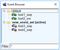
The top level objects are the event sets, and the children of these items are the event instances. The active event set is show in bold as shown above. There are unique icons to represent the current status of the event instances:
■Defined  - Event is defined but has not be executed yet
- Event is defined but has not be executed yet■Files on Disk  - Event files are on disk but no analysis has been executed
- Event files are on disk but no analysis has been executed■Files Successful  - Event files including analysis are on disk, and the analysis was successful
- Event files including analysis are on disk, and the analysis was successful■Files Failed  - Event files including analysis are on disk, but the analysis was not successful
- Event files including analysis are on disk, but the analysis was not successful■In Session Successful  - Event was executed, analysis is in session and was successful
- Event was executed, analysis is in session and was successful■In Session Failed  - Event was executed, analysis is in session but was not successful
- Event was executed, analysis is in session but was not successfulRight-click Menus
When you click right mouse button, different shortcut menus appear depending on the entity selected in the Model Browser. These menus are documented in detail in the Event Browser dialog box help.
Filter
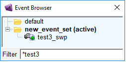
Event instance objects displayed in the event browser can be filtered by entering search strings in the Filter field:
Open-Loop Steering Events
Adams Car provides a wide range of open-loop steering analyses. In open-loop steering analyses, the steering input to your full vehicle is a function of time.
The open-loop steering analyses include:
Drift Analysis
In a drift analysis, the vehicle reaches a steady-state condition in the first ten seconds. A steady-state condition is one in which the vehicle has the desired steer angle and initial velocity values. In seconds 1 through 5 of the analysis, Adams Car ramps the steering angle/length from the initial value to the desired value using a STEP function. In seconds 5 through the desired end time, it linearly ramps the throttle at the desired ramp rate.
Note: | Adams Car creates an event file (.xml) that defines the analysis and the different parameters. It uses the .xml file for the analysis and then leaves it in the working directory so you can refer to it as needed. |
To set up a drift analysis:
1. From the Simulate menu, point to Full-Vehicle Analysis, point to Open-Loop Steering Events, and then select Drift.
2. Enter the necessary parameters as explained in the dialog box help for Full-Vehicle Analysis: Drift.
3. Select OK.
Fish-Hook Analysis
You use a fish-hook analysis to evaluate dynamic roll-over vehicle stability.
A fish-hook analysis consists of two mini-maneuvers (see Creating Mini-Maneuvers):
■A quasi-static phase sets up the vehicle at the desired initial conditions.
■The mini-maneuver runs the actual fish-hook analysis in which Adams Car computes the steering signal as a combination of step functions, and disengages the clutch. The maneuver provides a basis for evaluating a vehicle's transitional response and dynamic roll-over stability. The most important factors for this evaluation are: steering-wheel angle, lateral acceleration, yaw rate, and roll angle.
Adams Car conducts the analysis by driving at a constant speed, putting the vehicle in neutral, and turning one direction in a preselected steering-wheel angle and then turning the opposite direction in another preselected steering-wheel angle.
To set up a fish-hook analysis:
1. From the Simulate menu, point to Full-Vehicle Analysis, point to Open-Loop Steering Events, and then select Fish Hook.
2. Enter the necessary parameters as explained in the dialog box help for Full-Vehicle Analysis: Fish Hook.
3. Select OK.
Frequency Response Analysis
The goal of a frequency response analysis is to provide steering input that spans the entire frequency range of a human driver, roughly 0 to 3 Hz. The event determines either the steering wheel angle (SWA) required attaining a certain lateral acceleration (typically 0.3 g) at a given speed or you can specify SWA directly.
The sinusoidal amplitude either determined by the event or specified by user for the steering input. The frequencies are varies from zero to the maximum attainable (approximately 3.0 Hz). The most important quantities to be measured are:
■Lateral acceleration
■Yaw rate
■Roll angle
■Steering wheel torque
■Steering wheel angle
To set up a frequency response analysis:
1. From the Simulate menu, point to Full-Vehicle Analysis, point to Open-Loop Steering Events, and then select Frequency Response.
2. Enter the necessary parameters as explained in the dialog box help for Full-Vehicle Analysis: Frequency Response.
3. Select OK.
Note: | The frequency response analysis with input type as a swept sine would generate an excessive amount of output and be quite time consuming. An alternative is the input type as a pulse steer. A pulse steering input is applied, typically with a duration of 0.3 seconds and an amplitude of 60 to 120 degrees. Pulse steering inputs have excellent frequency content in the range of interest. If the vehicle response is kept within the linear handling range, the pulse steer option is a very efficient method of evaluating a vehicle's frequency response. |
Grist Mill Analysis
You use a grist mill analysis to evaluate the wheel loads and tire characteristics in a large steering angle steady state condition.
A grist mill analysis consists of two mini-maneuvers (see Creating Mini-Maneuvers):
■A quasi-static phase sets up the vehicle at the desired initial conditions.
■The mini-maneuver runs the actual grist mill analysis by driving the vehicle at a constant speed, with a steering ramped from zero to a specified value.
The most important factors for this evaluation are:
■Steady state wheel loads
■Wheel moments
■Rolling radius
■Slip angle
■Inclination angle
To set up a grist mill analysis:
1. From the Simulate menu, point to Full-Vehicle Analysis, point to Open-Loop Steering Events, and then select Grist Mill.
2. Enter the necessary parameters as explained in the dialog box help for Full-Vehicle Analysis: Grist Mill.
3. Select OK.
Hands Free Analysis
You use a hands free analysis to evaluate transient handling properties of a vehicle at limit handling conditions.
A hands free analysis consists of two mini-maneuvers (see Creating Mini-Maneuvers):
■A quasi-static phase sets up the vehicle at the desired initial conditions.
■The mini-maneuver runs the actual hands free analysis by driving the vehicle at a constant speed, with a sinusoidal steering input and deactivating steering input at a specified input angle.
The time at which to start the free hand event is based on the angle at which the steering input needs to be deactivated and the frequency of the steering input.
The most important factors for this evaluation are:
■Lateral acceleration.
■Steering wheel angle/torque.
■Yaw rate.
■Roll Angle
To set up a hands free analysis:
1. From the Simulate menu, point to Full-Vehicle Analysis, point to Open-Loop Steering Events, and then select Hands Free.
2. Enter the necessary parameters as explained in the dialog box help for Full-Vehicle Analysis: Hands Free.
3. Select OK.
Impulse-Steer Analysis
In an impulse-steer analysis, the steering demand is a force/torque, single-cycle, sine input. The steering input ramps up from an initial steer value to the maximum steer value. You can run with or without cruise control. The purpose of the test is to characterize the transient response behavior in the frequency domain.
Typical metrics are: lateral acceleration, and vehicle roll and yaw rate, both in time and frequency domain.
To set up a impulse-steer analysis:
1. From the Simulate menu, point to Full-Vehicle Analysis, point to Open-Loop Steering Events, and then select Impulse Steer.
2. Enter the necessary parameters as explained in the dialog box help for Full-Vehicle Analysis: Impulse Steer.
3. Select OK.
J-Turn Analysis
You use a J-Turrn analysis to evaluate the roll-over vehicle stability at limit handling condition..
A J-Turn analysis consists of two mini-maneuvers (see Creating Mini-Maneuvers):
■A quasi-static phase sets up the vehicle at the desired initial conditions.
■The mini-maneuver runs the actual J-Turn analysis by driving the vehicle at a constant speed, with specified steering wheel angle and steer rate. The maneuver provides a basis for evaluating a vehicle's transitional response and dynamic roll-over vehicle stability in the limit handing condition.
The most important factors for this evaluation are:
■Steering-wheel angle
■Lateral acceleration
■Yaw rate
■Side slip angle
■Roll angle
To set up a J-Turn analysis:
1. From the Simulate menu, point to Full-Vehicle Analysis, point to Open-Loop Steering Events, and then select J-Turn.
2. Enter the necessary parameters as explained in the dialog box help for Full-Vehicle Analysis: J-Turn.
3. Select OK.
On Center Analysis
The On Center analysis is used as the primary method to measure steering feel properties. The On Center control subroutine is used to calculate steering wheel angle required to achieve specified lateral acceleration.
This analysis requires two user defined variable statements in the dataset (on_center_var_1 and on_center_var_2). These variables are used to store the maximum lateral acceleration recorded during the first and second stage of the on center analysis. Based on these recorded lateral accelerations and the user specified steering wheel input for the first two stages of the analysis, the necessary steering wheel angle required to produce the user specified lateral acceleration can be determined.
For additional information refer, On Center.
To set up an on center analysis:
1. From the Simulate menu, point to Full-Vehicle Analysis, point to Open-Loop Steering Events, and then select On Center.
2. Enter the necessary parameters as explained in the dialog box help for Full-Vehicle Analysis: On Center.
3. Select OK.
Parking Effort Analysis
You use a parking effort analysis to evaluate the steering effort required for zero speed or low speed.
A parking effort analysis consists of two mini-maneuvers (see Creating Mini-Maneuvers):
■A quasi-static phase sets up the vehicle at the desired initial conditions.
■The mini-maneuver runs the actual parking effort analysis by driving the vehicle at a zero or low speed, with specified steering input. The maneuver provides a basis for evaluating a parking effort. The most important factors for this evaluation is: steering-wheel torque.
To set up a parking effort analysis:
1. From the Simulate menu, point to Full-Vehicle Analysis, point to Open-Loop Steering Events, and then select Parking Effort.
2. Enter the necessary parameters as explained in the dialog box help for Full-Vehicle Analysis: Parking Effort.
3. Select OK.
Ramp-Steer Analysis
In a ramp-steer analysis, you obtain time-domain transient response metrics. The most important quantities to be measured are: steering-wheel angle, yaw angle speed, vehicle speed and lateral acceleration. During a ramp-steer analysis, Adams Car ramps up the steering input from an initial value at a specified rate.
To set up a ramp-steer analysis:
1. From the Simulate menu, point to Full-Vehicle Analysis, point to Open-Loop Steering Events, and then select Ramp Steer.
2. Enter the necessary parameters as explained in the dialog box help for Full-Vehicle Analysis: Ramp Steer.
3. Select OK.
Single Lane-Change Analysis
During a single lane-change analysis, the steering input goes through a complete sinusoidal cycle over the specified length of time. The steering input can be:
■Length, which is a motion applied to the rack of the steering subsystem.
■Angle, which is angular displacements applied to the steering wheel.
■Force applied to the rack.
■Torque applied to the steering wheel.
To set up a single lane-change analysis:
1. From the Simulate menu, point to Full-Vehicle Analysis, point to Open-Loop Steering Events, and then select Single Lane Change.
2. Enter the necessary parameters as explained in the dialog box help for Full-Vehicle Analysis: Single Lane Change.
3. Select OK.
Sine with Dwell Analysis
During a sine with dwell analysis, the steering input goes through a sinusoidal cycle of specified frequency with specified dwell time after 75-percentage completion of the sinusoidal cycle. The steering input is an angle that is angular displacement applied to the steering wheel and is varies based on the specified increment of steering wheel angle. The number of tests run changes based on the specified inputs.
The most important factors for this evaluation are:
■Steering-wheel angle
■Lateral displacement
■Peak yaw rate
During a sine with dwell analysis, a quasi-static phase sets up the vehicle at the desired initial conditions and then a steering wheel angle is applied.
The maneuver provides a basis for evaluating a vehicle's transitional response and dynamic vehicle stability in the limit handing condition.
To set up a sine with dwell analysis:
1. From the Simulate menu, point to Full-Vehicle Analysis, point to Open-Loop Steering Events, and then select Sine with Dwell.
2. Enter the necessary parameters as explained in the dialog box help for Full-Vehicle Analysis: Sine with Dwell.
3. Select OK.
Step Steer Analysis
A step steer analysis yields time-domain transient-response metrics. The most important quantities to be measured are:
■Steering-wheel angle
■Yaw rate
■Vehicle speed
■Lateral acceleration
During a step steer analysis, Adams Car increases the steering input from an initial value to a final value over a specified time.
To set up a step steer analysis:
1. From the Simulate menu, point to Full-Vehicle Analysis, point to Open-Loop Steering Events, and then select Step Steer.
2. Enter the necessary parameters as explained in the dialog box help for Full-Vehicle Analysis: Step Steer.
3. Select OK.
Swept Steer Analysis
In swept steer analysis, steering inputs at the steering wheel let you measure a vehicles directional response characteristics under quasi-steady state turning condition. This provides a basis for evaluating a vehicle understeer gradient, roll gradient, steering sensitivity, lateral load transfer distribution.
The most important factors for this evaluation are:
■Steering-wheel angle
■Lateral acceleration
■Yaw rate
■Roll angle
During a swept steer analysis, Adams Car drive down a straight road at a constant speed and then a steering wheel angle is slowly applied until a specified lateral acceleration level is reached. For additional information refer, Swept Steer.
To set up a swept steer analysis:
1. From the Simulate menu, point to Full-Vehicle Analysis, point to Open-Loop Steering Events, and then select Swept Steer.
2. Enter the necessary parameters as explained in the dialog box help for Full-Vehicle Analysis: Swept Steer.
3. Select OK.
Swept-Sine Steer Analysis
Sinusoidal steering inputs at the steering wheel let you measure frequency-response vehicle characteristics. This provides a basis for evaluating a vehicle transitional response, the intensity and phase of which varies according to the steering frequency. The most important factors for this evaluation are:
■Steering-wheel angle
■Lateral acceleration
■Yaw rate
■Roll angle
During a swept-sine steer analysis, Adams Car steers the vehicle from an initial value to the specified maximum steer value, with a given frequency. It ramps up the frequency of the steering input from the initial value to the specified maximum frequency with the given frequency rate.
To set up a swept-sine steer analysis:
1. From the Simulate menu, point to Full-Vehicle Analysis, point to Open-Loop Steering Events, and then select Swept-Sine Steer.
2. Enter the necessary parameters as explained in the dialog box help for Full-Vehicle Analysis: Swept-Sine Steer.
3. Select OK.
Notes: | The Sinusoidal Steering analysis can be simulated as a special case of Swept-Sine Steer analysis. In sinusoidal steering analysis, the vehicle is simulated at constant speed with harmonic steering motion. The most important factors for this evaluation are: ■Steering-wheel angle ■Peak Lateral acceleration ■Peak Yaw rate ■Peak Roll angle ■Peak Side Slip Angle During a sinusoidal steering analysis, Adams Car drive down a straight road at a constant speed and steers with harmonic motion at user specified amplitude and frequency. To simulate sinusoidal steering analysis, specify Maximum Frequency = Initial Frequency and Frequency Rate =1. |
Turn Diameter Analysis
In turn diameter analysis, by using user defined or default inside and outside or single locations, let you measure the turn diameter of the vehicle.
The request "turn_diameter" created during analysis helps you measures the diameter for the inside, outside, and/or user-defined reference point for the turning circle.
The analysis applies a step function based on the specified steering amplitude or rack travel, and holds this value as the vehicle maneuvers through a circle.
To set up a turn diameter analysis:
1. From the Simulate menu, point to Full-Vehicle Analysis, point to Open-Loop Steering Events, and then select Turn Diameter.
2. Enter the necessary parameters as explained in the dialog box help for Full-Vehicle Analysis: Turn Diameter.
3. Select OK.
Cornering Events
You use cornering analyses to evaluate your vehicle's handling and dynamic responses during various cornering-type maneuvers. Cornering analyses use both open- and closed-loop controllers of the steering, throttle, brake, gear, and clutch signals to investigate various vehicle behaviors. You can investigate both steady-state and limit cornering to characterize responses such as understeer/oversteer gradients, weight transfer, and so on.
Note: | Adams Car creates an event file (.xml) that defines the analysis. The Driving Machine uses the event file to control the vehicle. Adams Car stores the event file in the working directory so you can refer to it as needed and examine it using the Event Builder. |
The cornering analyses include:
Braking-In-Turn Analysis
The braking-in-turn analysis is one of the most critical analyses encountered in everyday driving. This analysis examines path and directional deviations caused by sudden braking during cornering. Typical results collected from the braking-in-turn analysis include lateral acceleration, variations in turn radius, and yaw angle as a function of longitudinal deceleration.
In a braking-in-turn analysis, you can set the Driving Machine to drive your full vehicle, as follows:
■Drive down a straight road, turn onto a skidpad, and then accelerate to achieve a desired lateral acceleration
■Run a quasi-static skidpad setup, which places the vehicle on a skidpad with predefined lateral acceleration
The Driving Machine holds the longitudinal speed and radius constant for a time to let any transients settle. It then applies a brake signal to the vehicle to control the vehicle deceleration at a constant rate (units in g).
Depending on the controller type, the Driving Machine does either of the following:
■Open-loop - Locks the steering wheel
■Closed-loop - Maintains the skidpad radius
The Driving Machine maintains the braking for the given duration of the maneuver or until the vehicle speed drops below 2.5 meters/second.
You can use the plot configuration file, mdi_fva_bit.plt, in the shared Adams Car database to generate the plots that are typically of interest for this type of analysis.
To set up a braking-in-turn analysis:
1. From the Simulate menu, point to Full-Vehicle Analysis, point to Cornering Events, and then select Braking-In-Turn.
2. Enter the necessary parameters as explained in the dialog box help for Full-Vehicle Analysis: Braking-In-Turn.
3. Select OK.
Constant-Radius Cornering Analysis
For constant-radius cornering analysis, the Driving Machine drives your full vehicle down a straight road, turns onto a skidpad, and then gradually increases velocity to build up lateral acceleration. One common use for a constant radius cornering analysis is to determine the understeer characteristics of the full vehicle.
To set up a constant-radius cornering analysis:
1. From the Simulate menu, point to Full-Vehicle Analysis, point to Cornering Events, and then select Constant Radius Cornering.
2. Enter the necessary parameters as explained in the dialog box help for Full-Vehicle Analysis: Constant-Radius Cornering.
3. Select OK.
Cornering with Steer Release Analysis
The vehicle performs a dynamic constant-radius cornering to achieve the prescribed conditions (radius and longitudinal velocity or longitudinal velocity and lateral acceleration). After the steady state prephase, the steering wheel closed-loop signal is released, simulating a release of the steering wheel. The analysis focuses primary on the path deviation, yaw characteristics, steering-wheel measurements, roll angle, roll rate, and side-slip angle.
To set up an analysis of cornering with steer release:
1. From the Simulate menu, point to Full-Vehicle Analysis, point to Cornering Events, and then select Cornering w/Steer Release.
2. Enter the necessary parameters as explained in the dialog box help for Full-Vehicle Analysis: Cornering Steer Release.
3. Select OK.
Lift-off Turn-in Analysis
This analysis examines path and directional deviations caused by suddenly lifting the throttle pedal during cornering and applying an additional ramp steering input. Typical results collected from the lift-off turn-in analyses include lateral acceleration, variations in turn radius, and yaw angle as a function of longitudinal deceleration. Adams Car drives the vehicle through two distinct phases:
■Cornering pre-phase: Adams Car uses quasi-static calculations to set the vehicle at the correct initial conditions for the desired lateral acceleration at the given radius.
■Lift-off turn-in: The steer is ramped from the last value of the previous mini-maneuver at the desired rate. The throttle signal is set to zero; the clutch can be engaged or disengaged.
To set up a lift-off turn-in analysis:
1. From the Simulate menu, point to Full-Vehicle Analysis, point to Cornering Events, and then select Lift-Off Turn-In.
2. Enter the necessary parameters as explained in the dialog box help for Full-Vehicle Analysis: Lift-Off Turn-In.
3. Select OK.
Power-off Cornering Analysis
The purpose of this maneuver is to determine the power-off effect on course holding and directional behavior of a vehicle, whose steady-state circular path is disturbed only by power-off. The Driving Machine drives the vehicle through two distinct phases:
■An initial quasi-static setup that achieves the initial conditions.
■A power-off event where the throttle signal is stepped down from the value of the previous mini-maneuver to zero.
The lateral acceleration and skidpad radius define the initial conditions. Note that the significance of the results decreases with the skidpad radius. After reaching the initial steady-state driving conditions, the steering signal is kept constant and the accelerator pedal is released with a step signal profile. The release of the accelerator pedal is considered as the moment of power-off initiation, which you can define.
Typical results collected from power-off cornering analyses include variations in the heading direction and longitudinal deceleration, as well as side-slip angle, yaw angle, and gradient.
To set up a power-off cornering analysis:
1. From the Simulate menu, point to Full-Vehicle Analysis, point to Cornering Events, and then select Power-off Cornering.
2. Enter the necessary parameters as explained in the dialog box help for Full-Vehicle Analysis: Power-Off Cornering.
3. Select OK.
Throttle-On-In-Turn Analysis
The throttle-on-in-turn analysis is one of the most critical analyses encountered in everyday driving. This analysis examines path and directional deviations caused by sudden throttle during cornering.
The most important factors for this evaluation are:
■Lateral acceleration
■Variations in turn radius
■Yaw angle as a function of longitudinal deceleration
In a throttle-on-in-turn analysis, you can set the Driving Machine to drive your full vehicle, as follows:
■Drive down a straight road, turn onto a skidpad, and then accelerate to achieve a desired lateral acceleration
■Run a quasi-static skidpad setup, which places the vehicle on a skidpad with predefined lateral acceleration
The Driving Machine holds the longitudinal speed and radius constant for a time to let any transients settle. It then applies a throttle signal to the vehicle to control the vehicle acceleration at a constant rate (units in g).
Depending on the controller type, the Driving Machine does either of the following:
■Open-loop - Locks the steering wheel
■Closed-loop - Maintains the skidpad radius
The Driving Machine maintains the throttle for the given duration of the maneuver.
You can use the plot configuration file, mdi_fva_tit.plt , in the shared Adams Car database to generate the plots that are typically of interest for this type of analysis.
To set up a braking-in-turn analysis:
1. From the Simulate menu, point to Full-Vehicle Analysis, point to Cornering Events, and then select Throttle-on-In-Turn.
2. Enter the necessary parameters as explained in the dialog box help for Full-Vehicle Analysis: Throttle-On-In-Turn.
3. Select OK.
Straight-Line Events
The analyses based on the Driving Machine focus on the longitudinal dynamics of the vehicle. Adams Car uses open- and closed-loop longitudinal controllers to drive your vehicle model.
Note: | Adams Car creates an event file (.xml) that defines the analysis and the different parameters. It uses the .xml file for the analysis and then leaves it in the working directory so you can refer to it as needed. |
The straight-line-behavior analyses include:
Acceleration Analysis
During an acceleration analysis, the Driving Machine ramps the throttle demand from zero at your input rate (open loop) or you can specify a desired longitudinal acceleration (closed loop). You can specify either free, locked, or straight-line steering. An acceleration analysis helps you study the anti-lift and anti-squat properties of a vehicle.
To set up an acceleration analysis:
1. From the Simulate menu, point to Full-Vehicle Analysis, point to Straight-Line Behavior, and then select Acceleration.
2. Enter the necessary parameters as explained in the dialog box help for Full-Vehicle Analysis: Acceleration.
3. Select OK.
Brake Drift Analysis
During a brake drift analysis, the Driving Machine lets you specify a longitudinal deceleration (closed loop). You can vary side to side front brake split (brake bias) and road bank angle. You can also specify either free or locked steering. The brake drift analysis helps you to determine:
■Camber, caster and toe change for insight into the tire wear performance of the vehicle
■Front and rear dive/lift to identify antidive/antisquat performance during braking
■Brake drift (vehicle lateral displacement) from the time the brakes are applied to the completion of the simulation
To set up a brake drift analysis:
1. From the Simulate menu, point to Full-Vehicle Analysis, point to Straight-Line Behavior, and then select Brake Drift.
2. Enter the necessary parameters as explained in the dialog box help for Full-Vehicle Analysis: Brake Drift.
3. Select OK.
Braking Analysis
During a braking analysis, the Driving Machine ramps the brake input from zero at your input rate or lets you specify a longitudinal deceleration (closed loop). You can also specify either free or locked steering. The braking test analysis helps you study the brake-pull anti-lift and anti-dive properties of a vehicle.
To set up a braking analysis:
1. From the Simulate menu, point to Full-Vehicle Analysis, point to Straight-Line Behavior, and then select Braking.
2. Enter the necessary parameters as explained in the dialog box help for Full-Vehicle Analysis: Braking.
3. Select OK.
Braking on Split µ Analysis
During a braking on split µ analysis, the Driving Machine ramps the brake input from zero at your input rate while the left and right tires are on road segments with different road friction. You can also specify either free or locked steering. The braking on split µ test analysis helps you study the behavior of active brake, damper and traction controllers in a vehicle.
To set up a braking on split µ analysis:
1. From the Simulate menu, point to Full-Vehicle Analysis, point to Straight-Line Behavior, and then select Braking on Split µ.
2. Enter the necessary parameters as explained in the dialog box help for Full-Vehicle Analysis: Braking on Split µ.
3. Select OK.
Cross Wind Analysis
This analysis allows you to examine operating behavior and directional deviations caused by the effect of crosswind during a straight-line analysis. You need to specify proper aerodynamic coefficients into the aerodynamic force.
The most important factors for this evaluation are:
■Steering wheel torque
■Lateral acceleration
■Yaw rate
■Roll angle
During a cross wind analysis, Adams Car drives down a straight road at a constant speed and then a cross wind is applied for user specified distance or duration manually or by using wind file.
To set up a cross wind analysis:
1. From the Simulate menu, point to Full-Vehicle Analysis, point to Straight-Line Events, and then select Cross Wind
2. Enter the necessary parameters as explained in the dialog box help for Full-Vehicle Analysis: Cross Wind.
3. Select OK.
Maintain Analysis
During a maintain analysis, the Driving Machine either controls the throttle signal to maintain a constant longitudinal velocity, or holds the throttle demand constant (open loop). You can specify either free, locked, or straight-line steering. A maintain analysis helps you study the drive controller behavior for the properties of your vehicle model, and identify transient effects not active during static vehicle set-up pre-phase.
To set up a maintain analysis:
1. From the Simulate menu, point to Full-Vehicle Analysis, point to Straight-Line Behavior, and then select Maintain.
2. Enter the necessary parameters as explained in the dialog box help for Full-Vehicle Analysis: Maintain.
3. Select OK.
Power-off Straight Line Analysis
This analysis allows you to examine operating behavior and directional deviations caused by suddenly lifting off the throttle pedal during a straight-line analysis. Typical results collected from the power-off straight-line analysis include variations in heading direction and longitudinal deceleration. Optionally, you can depress the clutch during the throttle lift-off. In this case, you specify the duration that it takes to depress the clutch.
The Driving Machine drives the vehicle through two distinct phases:
■Quasi-static setup - The vehicle is set up in a straight line, to reflect the initial longitudinal velocity condition.
■Power-off event - The throttle signal is stepped down, from the value of the initial set mini-maneuver, to zero.
To set up a power-off straight line analysis:
1. From the Simulate menu, point to Full-Vehicle Analysis, point to Straight-Line Behavior, and then select Power-off Straight Line.
2. Enter the necessary parameters as explained in the dialog box help for Full-Vehicle Analysis: Power-Off Straight Line.
3. Select OK.
Steady State Drift Analysis
During a steady state drift analysis, the Driving Machine lets you specify a vehicle velocity. You can vary conicity force and torque, plysteer force and torque scale factor. You can also specify road bank angle. This analysis allows you to examine vehicle drift and suspension geometry changes during a straight line drive maneuver. The steady state drift test analysis helps you to determine:
■Camber, caster and toe change for insight into the tire wear performance of the vehicle
■Lateral vehicle drift (vehicle lateral displacement)
■Steering wheel torque and angle
■Left and right front lateral force change
To set up a steady state drift analysis:
1. From the Simulate menu, point to Full-Vehicle Analysis, point to Straight-Line Behavior, and then select Steady State Drift.
2. Enter the necessary parameters as explained in the dialog box help for Full-Vehicle Analysis: Steady State Drift.
3. Select OK.
Straight Line Drive Ride Analysis
This very similar to straight line maintain analysis. During a straight line drive ride analysis, the Driving Machine controls the throttle signal to maintain a constant longitudinal velocity, or holds the throttle demand constant (open loop, relative), or holds the throttle demand off (open loop, absolute). You can specify either free, locked, or straight-line steering. A straight line drive ride analysis helps you study the drive controller behavior for the properties of your vehicle model, and identify transient effects not active during static vehicle set-up pre-phase.
To set up a straight line drive ride analysis:
1. From the Simulate menu, point to Full-Vehicle Analysis, point to Straight-Line Behavior, and then select Straight Line Dive Ride.
2. Enter the necessary parameters as explained in the dialog box help for Full-Vehicle Analysis: Straight Line Drive Ride.
3. Select OK.
Course Events
Course analyses are based on the Driving Machine and are of a course-following type, such as ISO lane change.
In an ISO lane change analysis, the Driving Machine drives your full vehicle through a lane change course as specified in ISO-3888: Double Lane Change. You specify the gear position and speed at which to perform the lane change. The analysis stops after the vehicle travels 250 meters; therefore, the time to complete the lane change depends on the speed you specify.
The course analyses include:
Double Lane Change
During an ISO lane change analysis, a longitudinal controller maintains the chassis velocity to the desired value, and a lateral controller module acts on the steering system to maintain the vehicle on the desired ISO lane-change path.
Adams Car uses an external file to define the path for the maneuver: iso_lane_change.dcd defines the trace of the desired path on the x-y plane.
Note: | Adams Car creates an event file (.xml) that defines the analysis and the different parameters. It uses the .xml file for the analysis and then leaves it in the working directory so you can refer to it as needed. The file that defines the path is stored in the shared_car_database, in the driver_data table, and is called iso_lane_change.dcd. |
To set up an ISO lane change analysis:
1. From the Simulate menu, point to Full-Vehicle Analysis, point to Course Events, and then select ISO Lane Change.
2. Enter the necessary parameters as explained in the dialog box help for Full-Vehicle Analysis: Double Lane Change.
3. Select OK.
3D Road
A 3D road analysis simulates your vehicle assembly traversing a three-dimensional road representation and the obstacles or characteristics contained in that 3D road. The road file (.rdf/.xml) is used by both the tire subsystems to compute contact patch forces/moments, and by the lateral controller. The Driving Machine uses path information contained in the 3D road file to drive the vehicle along the specified course centerline. Example 3D road files are distributed in the shared Adams Car database (3d_road_*).
For more information about the 3D road, see Using the Road Builder.
To set up a 3D road analysis:
1. From the Simulate menu, point to Full-Vehicle Analysis, point to Course Events, and then select 3D Road.
2. Enter the necessary parameters as explained in the dialog box help for Full-Vehicle Analysis: 3D Road.
3. Select OK.
Roll Stability Events
Adams Car provides a range of events to analyse roll stability and simulate roll-over use cases.
The roll stability analyses include:
Embankment
During an embankment analysis, the vehicle is driven over a small ramp then down an embankment until it reaches the ground surface. The vehicle starts with an initial velocity and after the trigger point is passed and a specified delay is reached a constant ramp steer is applied. The steering stops at the final steering angle. The simulation ends when the end time is reached or the maximum roll angle is achieved (89 Deg.). The road can be used with or without rollover bar. The user can change the position and height of the rollover bar to meet his requirements. An embankment analysis helps you study the vehicle reactions to sliding down the road and rolling over. The embankment road type can be rigid or soft soil. The rollover bar is always rigid.
To set up an Embankment analysis:
1. From the Simulate menu, point to Full-Vehicle Analysis, point to Roll Stability Events, and then select Embankment.
2. Enter the necessary parameters as explained in the dialog box help for Full-Vehicle Analysis: Embankment.
3. Select OK.
Ramp (Corkscrew)
During a corkscrew analysis, the vehicle starts with an initial velocity and is driven over a ramp. The corkscrew dcp is similar to straight line maintain analysis. The simulation has three phases, ramp phase, airborne phase and ground sliding phase. The simulation ends when the end time is reached or the maximum roll angle is achieved. Corkscrew analysis helps you study the vehicle reactions to moving up and rolling over.
To set up a Ramp (corkscrew) analysis:
1. From the Simulate menu, point to Full-Vehicle Analysis, point to Roll Stability Events, and then select Ramp (Corkscrew).
2. Enter the necessary parameters as explained in the dialog box help for Full-Vehicle Analysis: Ramp (corkscrew).
3. Select OK.
Tilt Table Analysis
During the tilt table analysis, the vehicle is dynamically or quasi-statically tilted about the roll axis until the user specified tire force threshold is reached. A motion is applied to the tilt table to move the right side up or down. If the right side of the tilt table moves down, the right front wheel is constrained using an In line Primitive Joint (removes 2 translational DOFs), and the right rear wheel is constrained using an In plane Primitive Joint (removes 1 translational DOF). If the right side of the tilt table moves up the left wheels are constrained. This will prevent the vehicle from sliding in longitudinal and lateral direction. Also, each tire is constrained by a Perpendicular Primitive Joint to prevents the wheels from spinning (static solution). This test is used to estimate a vehicle's aggregate CG height and rollover point.
This event requires a full vehicle assembly with the Tilt Table Testrig.
To set up a Tilt Table analysis:
1. From the Simulate menu, point to Full-Vehicle Analysis, point to Roll Stability Events, and then select Tilt Table Analysis.
2. Enter the necessary parameters as explained in the dialog box help for Full-Vehicle Analysis: Tilt Table.
3. Select OK.
Sand Bed Analysis
The simulation starts with a quasi static till one second. During this time the table is adjusted to the tilt angle. After one second the analysis continues with the lateral initial velocity of the vehicle and ends at 2.5 seconds or a roll angle greater than 89 Degree. Using a model with the Tilt Table Testrig is required to run the simulation. Sandbed analysis helps you study the vehicle reactions to sliding down laterally and rolling over.
To set up a Sand Bed analysis:
1. From the Simulate menu, point to Full-Vehicle Analysis, point to Roll Stability Events, and then select Sand Bed (lateral).
2. Enter the necessary parameters as explained in the dialog box help for Full-Vehicle Analysis: Sand Bed (lateral).
3. Select OK.
Soft soil road types
The soft soil road types (soft soil, loose sand, lete sand for the embankment analysis and loose sand for the sand bed analysis) are only functional in combination with the FTire tire model.
More details about the pressure-sinkage and shear strength parameters for the various soil types used in FTire and based on the Bekker formulation can be found in the following reference: S.G. Mao, Ray P.S. Han, "Nonlinear complementarity equations for modeling tire-soil interaction - An incremental Bekker approach", Journal of Sound and Vibration 312 (2008) 380-398.
More information about the Cosin soft-soil models can be found in the Cosin Road Modeling Documentation at http://www.cosin.eu/res/cosinroad.pdf.
File-Driven Events
The file-driven analysis lets you run an analysis described in an existing event file (.xml).
Having direct access to event files lets you perform non-standard analyses on your full-vehicle assembly because all you have to do is generate a new event file describing the analysis.
To set up a file-driven analysis:
1. From the Simulate menu, point to Full-Vehicle Analysis, and then select File Driven Events.
2. Enter an Output Prefix.
3. If necessary, select a new Road Data File.
Press F1 for more detailed information on any of the selections in this dialog box.
4. Right-click in the Driver Control Files text box and select an XML Event file from the file selection dialog box.
5. Select OK.
Working with Event Files (.xml)
You use event files (.xml) to describe the maneuvers you want the Driving Machine to perform.
Event files (.xml) describe how you want the Driving Machine to drive your vehicle during a maneuver. The event file instructs the Driving Machine how fast to drive the vehicle, where to drive the vehicle (for example, on a 80 m radius skidpad), and when to stop the maneuver (for example, when lateral acceleration = 8 m/s2). Event files specify the kinds of controllers the Driving Machine should use for each of the available control signals (steering, throttle, brake, gear, and clutch). An event file can reference other files, primarily driver control data files (.dcd), to obtain necessary input data, such as speed versus time. Learn about referencing .dcd files.
Event files organize complex maneuvers into a set of smaller, simpler steps called mini-maneuvers. An event file defines the static-setup and a list of mini-maneuvers. For each mini-maneuver, the event file specifies how the Driving Machine is to control the steering, throttle, brake, gear, and clutch.
Learn about event files:
Creating Event Files
Before you can run a Driving Machine full-vehicle analysis, you must create (or use) an event file that contains one or more mini-maneuvers.
To set up Driving Machine mini-maneuvers:
1. From the Simulate menu, point to Full-Vehicle Analysis, and then select Event Builder.
The Event Builder dialog box has four major sections.
■File name, initial speed and gear, and units used in a selected field (shown at the bottom of the dialog box).
■Static Set-up and Gear Shifting Parameters.
■Mini-maneuver parameters on tabs for each of the five control signals with open-loop Control Value, plus an additional tab for Conditions to end a mini-maneuver.
■Closed-loop parameters (used when a control signal has its Control Method set to machine.
2. From the File menu, select New.
3. Enter the file name in the text box and click OK. The name appears in the Event File text box with a .xml extension. Initial default values appear in other text boxes.
4. If required, you can modify the initial Speed and Gear.
5. If required, you can modify values specified in the Static Set-up tab (for more information, see dialog box help for Event Builder).
6. Select the Gear Shifting Parameters tab. If required, you can modify values specified on this tab (for more information, see dialog box help for Event Builder).
7. If required, you can modify Machine Control control actions in the Trajectory Planning Parameter tab and Machine Control longitudinal and lateral PID Controller gains in the PID's Speed & Path and PID's Steering Output Parameters tabs (for more information, see dialog box help for Event Builder).
8. For MINI_1 (the default initial mini-maneuver), make selections for each of the control signal tabs (Steering, Throttle, Braking, Gear, and Clutch). Enter the necessary parameters as explained in the dialog box help for Event Builder to create the mini-maneuver.
9. Click the Conditions tab and enter the parameters required to end the mini-maneuver (for more information, see Specifying Conditions).
10. (Optional) Click the Linear tab and enter the parameters necessary to define any desired Linear analyses to be performed at the end of the mini-maneuver (for more information, see Specifying Linear Analyses).
11. To create additional mini-maneuvers, click the  button to the left of the mini-maneuver Name. This displays the Table Editor for mini-maneuvers.
12. In Table Editor mode, enter the name of your new mini-maneuver in the Name text box at the bottom of Event Builder.
13. Click Add. This adds a row to the Table Editor. You can edit any of the values in the row by clicking in the appropriate cell (for more information, see dialog box help for Event Builder).
14. Continue adding mini-maneuvers as necessary.
15. To return to Property Editor mode, either double-click a name (in the Name column), or select the name, right-click, and then select Modify with Property Editor.
16. When you've finished creating your event file, select Save.
After you create the file, you use it to run a file-driven analysis.
Learn about Structure of Event Files.
Using Event Files
After you use the Event Builder to create or modify an event file, you use that event file to run a file-driven analysis.
Creating Mini-Maneuvers
A mini-maneuver is a set of smaller, simpler analysis steps, such as a straight-line mini-maneuver. Mini-maneuvers are contained in event files (.xml).
To create a mini-maneuver, you must specify controls signals (steering, throttle, braking, gear, and clutch) and its conditions. For each control signal, you specify the following:
■Actuator type (steering only)
■Control method
■Control type
■Control mode
Learn more:
Specifying Actuators
Actuators specify custom actuators used when the Adams Car supplied actuation channels are not sufficient for the users needs.
The event file supports the following actuator UDEs in Adams Car:
■ac_joint_force_actuator
■ac_joint_motion_actuator
■ac_point_force_actuator
■ac_point_point_actuator
■ac_point_torque_actuator
■ac_variable_actuator
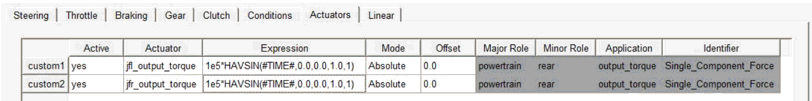
The Actuators tab of the Event Builder shows all actuators used by the current mini-maneuver. In Table Editor mode, you can see all defined actuators, select new actuators, modify actuator definitions, or remove actuators from the mini-maneuver.
Arguments
Label | Shows the actuator alias (not editable). |
Active | Sets the activity of the current actuator for the active mini-maneuver. |
Actuator | Adams Car populates this option menu with all the user-defined actuators available in the active model. Selecting an actuator from the list will populate the other fields with the current setting for that particular actuator. Note: Actuators of application type 'steering' and 'driver_demand' are not populated to not interfere with the driving machine. |
Expression | Function expression for the currently selected actuator. You can define functions of absolute time (for example, 1e5*HAVSIN(TIME,0,0,1,1)) or reference the value of a condition sensor in your expression by using #condition_sensor# (for example, 1e5*HAVSIN(#time#,0,0,1,1) for using the mini-maneuver time). You can also use the final value of a condition sensor of the previous mini-maneuver in your expression by using @condition_sensor@ (for example, @rack_travel@). |
Mode | Absolute indicates that the final value is absolute. Relative indicates that the final value is relative to the initial value. |
Offset | Offset value for the actuator. |
Major Role | Describes the major role of the parent of the actuator and is used to identify the actuator while populating the actuator table. |
Minor Role | Describes the minor role of the parent of the actuator and is used to identify the actuator while populating the actuator table. |
Application | Describes the purpose of the actuator and is used to identify the actuator while populating the actuator table. |
Identifier | Describes the actuator instance for the application area. |
Specifying an Actuator Type
When defining the steering control for a mini-maneuver, you must specify an actuator type. You use the actuator type to specify whether the Driving Machine steers the vehicle at the steering wheel or steering rack and whether the Driving Machine uses a force or motion. For example, when you set Actuator Type to rotation, the Driving Machine steers using a motion on the steering wheel.
The actuator type you select for steering determines how the Driving Machine interprets the units of other parameters associated with the steering signal. For example, if you set Actuator Type to torque, the Driving Machine interprets the amplitude argument for an open-loop sinusoidal input as torque (with units of length*force). If you set Actuator Type to rotation, however, the Driving Machine interprets the amplitude as an angle.
Arguments
force | Driving Machine steers the vehicle by applying a force to the steering rack. |
rotation | Driving Machine steers the vehicle using a MOTION statement on the steering-wheel revolute joint. |
torque | Driving Machine steers the vehicle by applying torque to the steering wheel. |
trans | Driving Machine steers the vehicle using a motion on the steering rack translational joint. |
Note: | Rotation and translation Actuator Types are implemented as motions. When Control Method is set to Machine (or SmartDriver) these motions necessarily depend on system states other than time. Such motions pose greater problems for some integrators than others in Adams. By default the driving machine detects and avoids using these Actuator Types with those integrators (automatically uses a torque actuator instead of a rotation actuator or a force actuator instead of a translation actuator.) Similarly, when Control Method is set to Open, some integrators benefit more than others if the function expression defining the open loop motion for rotation and translation Actuator Types is extracted and applied directly to the motion. By default, the driving machine detects these situations and applies extracted function expressions accordingly. These actions are taken at runtime, after the integrator setting is known. It is possible to override this behavior (to force the use of the originally selected actuator) by setting the environment variable MSC_ADAMS_VDM_SI2FLAG. |
Specifying a Control Method
When defining any mini-maneuver, you must specify a control method for each control signal.
Arguments
■Open
■Machine
■SmartDriver
Open Control Method
The Driving Machine output for the control signal is a function of time, and you must specify the function using the Control Type argument.
You cannot switch from an open-loop control mini maneuver to a SmartDriver mini maneuver. You can, however, switch from SmartDriver in a preceding mini maneuver to open-loop control in a subsequent mini maneuver.
Machine Control Method
Setting Control Method to machine specifies the vehicle path, speed profile, and other parameters used by machine control.
If you set machine control for gear and clutch, you must also supply the maximum and minimum engine speed. Machine control up-shifts to keep engine speed less than maximum and down-shifts to keep engine speed greater than minimum.
If you set Control Method to machine for steering, then you should specify the target path, using the Steer Control argument.
If you set Control Method to machine for throttle or brake, then you should specify the target speed profile, using the Speed Control argument.
Notes: | ■If you set Speed Control to lat_accel, then you must set Steer Control to skidpad. ■Machine control for clutch requires machine control for gear. If a manual powertrain is not used, the Control method for gear and clutch will be changed to open during the simulation if they are set to machine in the Event file. For the gear, the Adams Solver message file will show 'Drv_Vhl::ifInit Forcing open-loop gear behavior because powertrain has no gear input.' A similar message is shown for the clutch. |
Arguments
Steer Control | You can select one of the following: ■ay_s_map/ay_t_map - To define these closed-loop steering conditions, you can use a Table/Plot editor that you access by selecting the Table Editor button. ■file - ■File Name - Enter the name of a file that contains the path data. ■Lat. Path Offset - Allows driving at the specified lateral path offset (unit of length) to the path as provided by the road data file (for .xml, .rdf, .crg, .rgr file formats). ■path_map - To define this closed-loop steering condition, you can use a Table/Plot editor that you access by selecting the Table Editor button. To define this closed-loop steering condition, you can use a Table/Plot editor that you access by selecting the Table Editor button. ■skidpad - ■Entry Distance - Specifies the length of the straight path preceding the turn. Note that all paths are relative to the position of the vehicle at the end of the preceding mini-maneuver. If the preceding mini-maneuver was a skidpad and you want the vehicle to continue on the same circle in the current mini-maneuver, then specify zero (0) for Entry Distance. ■Radius - Specifies the radius of the skidpad. ■Turn Direction - Specifies which way the vehicle turns when traveling forward. ■straight - The vehicle travels forward from its current position along the tangent of the path from the preceding mini-maneuver. If the vehicle was under open-loop steering control in the preceding mini-maneuver, then the vehicle travels forward in the direction of its current velocity. You don't need to specify additional arguments. |
Speed Control | You can select one of the following: ■ax_s_map ■ax_t_map ■file ■File Name - Enter the name of a file that contains the closed-loop data. ■lat_accel - Be sure to set Steer Control to skidpad. ■Lat. Acc. - Enter a value for the lateral acceleration. ■lon_accel ■Start Time ■Long. Acc - Enter a value for the longitudinal acceleration. ■maintain - The Driving Machine maintains the speed of the vehicle at a value determined as follows: ■Velocity Type - If set to initial_actual, maintain the actual speed of the vehicle at the end of the preceding mini-maneuver or the initial speed set in the EXPERIMENT block if this mini-maneuver is the first in the experiment. If set to initial_target, maintain the target speed at the end of the preceding mini-maneuver if the preceding mini-maneuver was also using the machine Control Method for Throttle/Brake (this produces a continuous transition between two mini-maneuvers both using machine), otherwise the same as initial_actual. If set to specified, maintain the speed given by the Velocity field (see next.) ■Velocity - Maintain the specified speed, used only for Velocity Type = specified (see previous.) ■speed_s_map ■speed_t_map |
■vel_polynomial ■Velocity - Specifies the vehicle speed as polynomial of time. The Driving Machine computes the speed using the following relation: IF (Time < START_TIME): SPEED = VELOCITY IF ( TIME START_TIME ): SPEED = VELOCITY + ACCELERATION*(TIME - START_TIME)+ 1/2*JERK*(TIME-START_TIME)**2 where START_TIME is the starting time relative to the beginning of the mini-maneuver. Specify the following arguments: VELOCITY = value <length/time> ACCELERATION = value <length/time2> JERK = value <length/time3> START_TIME = value <time> Note that JERK is the time rate of change of acceleration. JERK = d(acceleration)/dt. ■Acceleration ■Jerk ■Start Time ■You can use a Table/Plot editor to define the various maps of speed and acceleration expressed as a function of time or distance traveled. |
SmartDriver Control Method
When you set Control Method to SmartDriver, you must also specify the Control Mode, the task, course file, as well as the maximum driving, braking, and turning accelerations.
Arguments
Task | Select one of the following: ■user_defined - Set your own vehicle limits. ■vehicle_limits - Use the maximum vehicle limits. |
Course File | Displays the name of a .xml or .drd file that describes the path over which the Driving Machine or Adams SmartDriver drive the vehicle. |
 | Select to choose a course file. |
Max Driving Acc | Enter the maximum driving acceleration index. Valid values are 0 to 100. |
Max LH Turn Acc | Enter the maximum left turn acceleration index. Valid values are 0 to 100. |
Max Braking Acc | Enter the maximum braking acceleration index. Valid values are 0 to 100. |
Max RH Turn Acc | Enter the maximum right turn acceleration index. Valid values are 0 to 100. |
Front Axle Coupling | Fraction of maximum available traction and steering force (tire-force ellipse) at front axle to utilize in generating static target speed profile (bigger values give more aggressive speed targets.) |
Rear Axle Coupling | Fraction of maximum available traction and steering force (tire-force ellipse) at rear axle to utilize in generating static target speed profile (bigger values give more aggressive speed targets.) |
Auto ICs For Vx | The "Speed" parameter for the Maneuver (including the Static Set-Up) will be replaced by SmartDriver with a value consistent with the target speed profile at the starting position of the vehicle on the target path. (Note, the target speed profile determined will not be constrained to begin at the Speed value specified for the Maneuver.) |
Auto ICs For Accx | The "Long Acc." parameter for Static Set-Up (the initial Acceleration for the Maneuver, including the Static Set-Up) will be replaced by SmartDriver with a value consistent with the target speed profile at the starting position of the vehicle on the target path. |
Auto ICs For Gear | The "Gear" parameter for the Maneuver (including the Static Set-Up) will be replaced by SmartDriver with a value consistent with the target speed profile at the starting position of the vehicle on the target path. |
Specifying a Control Type
For any of the control signals (steering, throttle, braking, and so on), when you set Control Method to open, Adams Car enables the Control Type option.
Arguments
constant | The Driving Machine inputs a constant signal to your vehicle model. ■Control Value - Enter a real number. |
data_driven | Specifies that the control signal comes from a driver control data file (.dcd), which you specify. The Driving Machine opens the .dcd file and reads the appropriate data. ■Dcd Filename - Enter the name of a .dcd file. |
data_map | Lets you specifies a series of discrete values as a function of time. Click the Open Loop Demand Map button that appears to enter values and view a plot of the values you enter. Note: The data provided will be interpolated linearly, and if extrapolated will saturate. |
function | Specifies that you should use any valid Adams Solver function expression based on time. ■Function - Enter a time-based function. For example: C20.0*SIN(2*PI*TIME) where TIME is the simulation time. |
impulse | The Driving Machine outputs an impulse to your vehicle constructed from a pair of cubic step functions. To define the impulse, you must specify the following arguments: ■Start Time - The starting time of the impulse relative to the beginning of the mini-maneuver. For example, if the mini maneuver starts at 1.2 seconds simulation time and Start Time = 0.3 seconds, then the impulse begins at 1.5 seconds simulation time. ■Duration - The length in time of the impulse. ■Maximum Value - The height of the impulse. The impulse reaches its maximum value relative to the start time at half the duration. Adams Car computes the IMPULSE function as follows: Let T1 = ( TIME - START_TIME ) / DURATION/2.0 Let T2 = ( TIME - (START_TIME + DURATION/2.0) ) / DURATION/2.0 IF ( T1 < 0.0 ): OUTPUT = 0.0 IF ( 0 < T1 < 1.0 ): OUTPUT = MAXIMUM_VALUE * ( 3.0 - 2.0*T1)*T1*T1 IF ( T1 > 1.0 and T2 < 1.0 ) OUTPUT = MAXIMUM_VALUE( 1.0 - (3.0 -2.0*T2)*T2*T2 ) IF ( T2 > 1.0 ); OUTPUT = 0.0 The following plot illustrates the IMPULSE function:  |
ramp | The Driving Machine supplies a ramp input. To define the ramp, you must supply the following arguments: ■Start Time ■Ramp Value Adams Car computes the RAMP function as follows: If ( time < START_TIME ) input = INITIAL_VALUE if ( time > START_TIME ) then input = INITIAL_VALUE + ( time - START_VALUE) * RAMP_VALUE Note: When using the RAMP function, the output value grows for the duration of the mini-maneuver. |
sine | The Driving Machine outputs a single-cycle sinusoid to your vehicle smoothed at the beginning and end by cubic-step functions. The duration of each cubic-step function is 1/100*CYCLE_LENGTH. ■Start Time - The starting time of the sinusoid relative to the beginning of the mini-maneuver. For example, if the mini-maneuver starts at 2.1 seconds simulation time and Start Time = 0.3 seconds, then the sinusoid begins at 2.4 seconds simulation time. ■Amplitude - The amplitude of the sinusoid. ■Cycle Length - The length of time to complete one cycle of the sinusoid. Adams Car computes the SINE function as follows: Let T1 = (TIME - START_TIME) / CYCLE_LENGTH / 100.0 Let T2 = (TIME - (START_TIME + 0.99*CYCLE_LENGTH)) / CYCLE_LENGTH / 100.0 IF ( T1 < 0.0 ): OUTPUT = INITIAL_VALUE IF ( 0 < T1 < 1.0 ): OUTPUT = INITIAL_VALUE + AMPLITUDE * SIN( 2.0*PI*(TIME - START_TIME)/ CYCLE_LENGTH) * (3.0 - 2.0*T1)*T1*T1 IF ( T1 > 1.0 and T2 < 0.0 ) OUTPUT = INITIAL_VALUE + AMPLITUDE * SIN( 2.0*PI*(TIME - START_TIME)/ CYCLE_LENGTH) IF ( T1 > 1.0 and 0.0 < T2 < 1.0 ) OUTPUT = INITIAL_VALUE + AMPLITUDE * SIN( 2.0*PI*(TIME - START_TIME)/ CYCLE_LENGTH) (1.0 - (3.0 -2.0*T2)*T2*T2) IF ( T2 > 1.0: OUTPUT = INITIAL_VALUE The following plot illustrates the SINE function: 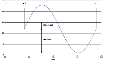 |
step | The Driving Machine inputs a STEP5 function to your vehicle model based on the following input parameters, which you must supply: ■Start Time ■Duration ■Final Value Adams Car computes the STEP5 function as follows: STEP5(time,START_TIME,INITIAL_VALUE,START_TIME+DURATION,FINAL_VALUE) Note that START_TIME is relative to the beginning of the mini-maneuver.  |
swept_sine | Sweeps the frequency of the output from the initial frequency to a maximum frequency at a given rate. Once the maximum frequency is achieved, the frequency remains constant. The amplitude of the swept sine function is fixed. To define swept sine, you must supply the following parameters: ■Start Time - The starting time of the function, measured from the beginning of the mini-maneuver. ■Amplitude - The amplitude of the swept-sine function. ■Initial Frequency - The starting frequency of the swept-sine function in <cycles/time>. ■Frequency Rate - The rate the frequency is swept from the initial frequency to the maximum frequency <cycles/time/time>. ■Max Frequency - The maximum frequency of the swept sine function in <cycles/time>. The following plot illustrates the SWEPT_SINE open-loop function:  |
Specifying a Control Mode
If you set Control Method to open, you must also define the Control Mode as either absolute or relative. If Control Method is not open, Control Mode is always absolute. With all open-loop maneuvers, the value of the preceding mini maneuver is used as the starting point for the next mini-maneuver. This is irrespective of whether you set Control Mode to relative or absolute. For example, your vehicle is driving on a skid pad at 30 mph, with 20o of steering wheel, when the first mini-maneuver is finished. The steering-wheel angle for the next mini maneuver will be 20o.
You can set Control Mode for the following open-loop control types:
■constant
■data_driven
■data_map
■step
For these control types, Control Mode changes the meaning of the FINAL_VALUE input in the .xml. Control Mode has no effect on the rest of the Control Types, nor on machine, and SmartDriver control methods.
The relative and absolute methods allow you to define the steering-wheel angle for the end of the next mini maneuver.
Arguments
Absolute | Indicates that the final value is absolute. For example, for a step input to the steering where the initial steering is 10 degrees and the final value is 50 degrees, the steer at the end of the step equals 50 degrees. |
Relative | Indicates that the final value is relative to the initial value. For example, for a step input to the steering where the initial steering is 10 degrees and the final value is 50 degrees, the steer at the end of the step equals 60 degrees. |
Here is another example. If at the beginning of the mini-maneuver the steering is 20o, the steering Control Method is set to open, the Control Type is set to step, and the FINAL_VALUE = 90.0, then FINAL_VALUE is relative to INITIAL_VALUE, and the steering angle at the end of the step input is 110o. If, however, Control Mode is set to Absolute, then the steering angle at the end of the step input equals the FINAL_VALUE of 90o
Specifying Conditions
Conditions specify when one mini-maneuver ends so the next one can begin. For example, you might end a mini-maneuver when the vehicle speed reaches 100 kph. You can also group end conditions together. For example, you might end a mini-maneuver when the vehicle speed reaches 100 kph and the lateral acceleration exceeds 5 m/s2.
The event file supports conditions based on time, distance, velocity, acceleration, and many other vehicle control variables. Conditions reference a measure or solver variable by name to measure a given quantity in the model.
The Conditions tab of the Event Builder shows one possible condition at a time in Property Editor mode. To add conditions or view other defined conditions, click the button to the left of the condition name to enter Table Editor mode. In Table Editor mode, you can see all defined conditions, add new conditions, modify conditions, or delete conditions. The Table Editor mode also lets you see the full set of arguments available for each condition.
Arguments
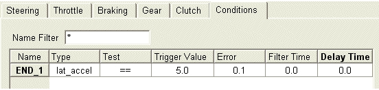
Then, the end condition is satisfied if:
5 - 0.1 < Lateral acceleration < 5 + 0.1
Name Filter | Filters the listed conditions based on the substring you specify. |
Name | Shows the condition name (not editable). |
Type | Quantity that is measured. Can be: ■curvature - Curvature of the vehicle trajectory ■distance - Total distance traveled by the vehicle during a mini-maneuver ■engine_speed - Angular velocity of the engine crankshaft in number of revolutions per minute (rpm) ■lat_accel - Vehicle lateral acceleration ■lat_dis - Vehicle lateral displacement with respect to the global reference system ■lat_velocity - Vehicle lateral velocity ■loc_accel - Vehicle longitudinal acceleration ■lon_dis- Vehicle longitudinal displacement with respect to the global reference system. ■pitch_angle - Angular displacement about the vehicle's lateral axis ■pitch_rate - Time derivative of pitch angle ■rack_tra_vel - Time derivative of rack displacement ■rack_travel - Displacement in the steering rack joint ■radius - Radius of vehicle trajectory ■roll_angle - Angular displacement about the vehicle's longitudinal axis ■roll_rate - Time derivative of vehicle roll angle ■side_slip_ang - Angle between the ground-plane projections of the vehicle's longitudinal axis and its velocity vector ■stee_ang_vel - Time derivative of steering angle ■steering ang - Angular displacement in the steering-wheel joint ■time - Simulation time ■user_defined - Allows you to create your own user-defined condition sensor. In the .xml event file, the dcf:DcfEndCondition -> userString holds the name of the condition sensor. ■velocity - Vehicle longitudinal velocity ■vert_accel - Vertical acceleration of driver reference frame with respect to origo marker ■vert_dis - Vehicle vertical displacement with respect to the global reference system ■vert_velocity - Vehicle vertical velocity with respect to the global reference system ■yaw_accel - Angular acceleration about the vehicle's vertical axis ■yaw_angle - Angular displacement about the vehicle's vertical axis ■yaw_rate - Angular velocity about the vehicle's vertical axis |
Test | ■== - Equal to trigger value ■>> - Greater than the trigger value ■<< - Less than the trigger value ■|==| - Absolute type value is equal to the trigger value ■|<<| - Absolute type value is less than the trigger value ■|>>| - Absolute type value is greater than the trigger value |
Trigger Value | The value against which the measure is tested to determine if the end condition is satisfied. Except for ENGINE_SPEED, which uses RPMs, you must specify the value in modeling units as defined in the event file. |
Error | The allowed difference between measure and value that still satisfies the test. Error must be positive and be specified in modeling units as defined in the event file (except engine_speed, which is in RPMs). For example, if the cells of the table are: |
Filter Time | The test must be satisfied continuously over the filter time to satisfy the end condition. filter time must be positive. |
Delay Time | Once the end condition is satisfied, delay the end of the mini-maneuver by delay time. |
Group Name | You specify a name to group conditions together. All conditions having the same group name must be satisfied simultaneously to end a mini-maneuver. For example, you might specify two end conditions: ■Longitudinal velocity equal to 20 m/s ■Lateral acceleration greater than 5 m/s/s Then you place the specified end conditions in the group mygroup. To end the mini-maneuver, the longitudinal velocity must be 20 m/s and the lateral acceleration must be greater than 5 m/s/s. |
Condition Type | Select a condition type: ■abort - When met, it causes the simulation to stop. ■end - When met, it causes the simulation to proceed to the next mini-maneuver, if one is defined. ■info - Not yet implemented ■warning - Not yet implemented |
Specifying Linear Analyses
Linear Analyses specify linearization type analyses that should be performed at the end of the mini-maneuver.
The event file supports any number of linear analyses of each of the four available types and all of the available options and arguments that are documented in the Adams Solver documentation.
The Linear tab of the Event Builder shows one linear analysis at a time in Property Editor mode. To add linear analyses or view other defined linear analyses, click the button to the left of the linear analysis name to enter Table Editor mode. In Table Editor mode, you can see all defined linear analyses, add new linear analyses, modify linear analyses, or delete linear analyses. The Table Editor mode also lets you see and modify a subset of arguments available for each linear analysis.
Arguments
Linear Analysis | Chooses the type of linear analysis to be performed, can be: ■Eigen Solution - calculate eigenvalues and eigenvectors ■ABCD Matrices - export state matrices ■MKB Matrices - export MKB matrices* ■BDF Export - export to Nastran* |
Include Damping | Dissipative effects can be included or excluded for Eigen Solution and MKB Matrices* |
Include Vectors | Eigen Solution can calculate eigenvalues only, or both eigenvalues and eigenvectors. |
Output Filename | Specify file name/prefix for ABCD Matrices, MKB Matrices* and BDF Export* |
Format | Specify exported file format for ABCD Matrices and MKB Matrices*, can be: ■Matlab - produce files suitable for Matlab import. ■MatrixX - produce files suitable for MatrixX import. |
BDF Type | Specify type of BDF export, can be: ■Closedbox - lumped ■Openbox - element-by-element |
Coordinates Table | Include a coordinates table for selected modes |
Dissipative Table | Include a dissipative energy table for selected modes |
Kinetic Table | Include a kinetic energy table for selected modes |
Strain Table | Include a strain energy table for selected modes |
Specify Tables by | Choose how to select modes for tables, can be: ■Modes - select by mode number ■Frequency - select by natural frequency* |
Use View Names | Tables can identify model elements using only Solver ids, or using Solver ids and View names* |
Precision | Specify number of significant digits in values in tables* |
Start Mode | Select modes starting with this mode number |
End Mode | Select modes ending with this mode number |
Start Frequency | Select modes with natural frequencies in the range Start Frequency - End Frequency* |
End Frequency | (see above) |
PINPUT | Specify the PINPUT statement to use when exporting ABCD or MKB* Matrices |
POUTPUT | Specify the POUTPUT statement to use when exporting ABCD or MKB* Matrices |
PSTATE* | Specify the PSTATE statement to use for Eigen Solution or when exporting ABCD or MKB* Matrices |
RM* | Specify the MARKER statement to use for Eigen Solution or when exporting ABCD or MKB* Matrices |
Config. File* | Specify the name of a configuration file to use for BDF Export |
* - these arguments are supported only in the C++ solver.
Referencing .dcd Files
You can reference driver control data (.dcd) files through XML event files to specify data for the method of control of the vehicle. When referencing .dcd files, event files can obtain two types of data:
■Open-loop data - Includes steering-wheel angle, throttle position, brake pressure, gear, and clutch position tabulated against time or distance traveled.
■Closed-loop data - Uses data from the dcd file to fix the vehicle path and speed for a mini-maneuver. Examples of closed-loop data are the vehicle position {x, y} versus time (t) or path {x, y} versus distance traveled (s). Closed-loop data can also include vehicle speed and lateral acceleration which the Machine Control integrates to determine the desired vehicle path and speed.
You reference .dcd files in your event files by selecting Machine for Steering/Throttle and Braking and browsing your databases for dcd files in the File Name text box. That is, using the file option for Machine Control means that you want to obtain control data from a .dcd file.
Example Event Files
In Adams Car, XML became the default file format for Driving Machine analyses. Although Adams Car still supports driver control files (.dcf), it now automatically converts them to .xml. The .xml files are referred to as event files. Although the contents of the two files types look different, they contain the same event information. You work with .xml files through the Event Builder.
In the shared Adams Car database, we provide files in both .dcf and .xml format. These files are stored in the driver_controls.tbl directory/table.
Switching mini-maneuver in real time
Running real time simulations, the time to switch between mini-maneuvers may result in a large runTime spike which among others are caused by initial condition operations executed immediately after switching to next mini-maneuver. You can significantly reduce the time to switch between mini-maneuvers by setting environment variable ADAMS_REALTIME_MINI_FAST (in combination with environment variable MSC_ADAMS_REAL_TIME = "ON"). As currently only variables are supported for fast mini transitions, you also need to set MSC_ADAMS_VDM_OPEN_EXPR = 0 which enforces using a VARSUB for the driver actuators.
When creating an FMU using the .fmd FMU definition file, please ensure that sensors are not removed from the model to prevent mini's from being skipped during the simulation: REMOVE_SENSORS = 'NO' under section [FMU_DEFINITION] in the .fmd file.
Also, the full driving machine should be used. When the event file only contains open-loop type of mini-maneuvers, the Driving Machine State is set to Open Loop Event and the driving machine GSE is not executed. This is not an issue if one of the mini-maneuvers has a machine controlled driving actuator.
To ensure that the full driving machine is used you can set FULL_DRIVING_MACHINE = 'YES' under section [FMU_DEFINITION] in the .fmd file.
Note: | Ensure that function expressions set on the actuators, such as steering, throttle, etc, through the .xml event files are continuous as no initial condition operations are performed, otherwise acceleration spikes may occur. |
Static and Quasi-Static Analyses
Static and Quasi-static analyses find dynamic equilibrium solutions for your full vehicle at increasing, successive values of lateral and/or longitudinal acceleration. Static and Quasi-static analyses, in contrast to open-loop and closed-loop analyses, do not include transient effects and solve very quickly. For example, in a quasi-static analysis, a change in lateral acceleration from 0.1g to 0.5g does not show the lateral acceleration or yaw rate overshoot that a similar open-loop and closed-loop analysis might show.
The following topics contain information on setting up quasi-static analyses, as well as a description of the types of quasi-static analyses:
Quasi-Static Constant-Radius Cornering Analysis
You perform a constant radius cornering analysis to evaluate your full vehicle's understeer and oversteer characteristics. The constant radius cornering analysis holds the turn radius constant and varies the vehicle velocity to produce increasing amounts of lateral acceleration.
This analysis:
■Uses a force-moment method to balance the static forces to 0 at each time step.
■Provides a faster solution than the corresponding dynamic analysis, but doesn't account for transient effects, such as gear shifting.
■Can be useful when exploring the limit handling characteristics of the vehicle due to a combination of both the longitudinal and lateral acceleration.
■Differs from the constant-velocity cornering analysis in that the turn radius is fixed and the longitudinal velocity varies.
A CONSUB controls this analysis. For more information on CONSUB, see Welcome to Adams Solver Subroutines.
You can, for example, use the plot configuration file, mdi_fva_ssc.plt, in the shared Adams Car database to generate the plots that are typically of interest for this analysis. Otherwise, in Adams PostProcessor, you can create your own plots by selecting the desired requests and components.
To set up a constant-radius cornering analysis:
1. From the Simulate menu, point to Full-Vehicle Analysis, point to Static and Quasi-Static Maneuvers, and then select Constant-Radius Cornering.
2. Enter the necessary parameters as explained in the dialog box help for Quasi-Static Constant Radius Cornering.
3. Select OK.
Quasi-Static Constant-Velocity Cornering Analysis
You perform a constant velocity cornering analysis to evaluate your full vehicle's understeer and oversteer characteristics. The constant velocity cornering analysis holds the vehicle velocity constant and varies the turn radius to produce increasing amounts of lateral acceleration. The input parameters for this analysis are similar to the steady-state cornering analysis except that you specify the vehicle longitudinal velocity instead of the turn radius.
This analysis:
■Uses a force-moment method to balance the static forces to 0 at each time step.
■Provides a faster solution than the corresponding dynamic analysis, but doesn't account for transient effects.
■Can be useful when exploring the limit handling characteristics of the vehicle due to a combination of decreasing turn radius and longitudinal acceleration.
■Differs from the constant-radius cornering analysis in that the turn radius is not fixed.
If your powertrain model is based on a General State Equation subroutine (that is, derived from and compatible with one of the shared powertrain template examples), this event will use the throttle to achieve the desired longitudinal acceleration. If you specify a negative longitudinal acceleration, the throttle will be used to control engine braking and thus deceleration, unless the additional power of the brakes is required to achieve the desired deceleration.
A CONSUB controls this analysis. For more information on CONSUB, see Welcome to Adams Solver Subroutines.
You can use the plot configuration file, mdi_fva_ssc.plt, in the shared car database to generate the plots that are typically of interest for this analysis.
To set up a constant-velocity cornering analysis:
1. From the Simulate menu, point to Full-Vehicle Analysis, point to Static and Quasi-Static Maneuvers, and then select Constant-Velocity Cornering.
2. Enter the necessary parameters as explained in the dialog box help for Quasi-Static Constant Velocity Cornering.
3. Select OK.
Quasi-Static Force-Moment Analysis
You perform a force-moment analysis to evaluate the stability and handling characteristics of your vehicle model. During the analysis, Adams Car drives the vehicle at constant longitudinal speed and performs a series of analyses at different side-slip angles and steer angles. The analysis:
■Represents a typical test in which the vehicle is constrained on a model flat-belt tire tester.
■Is based on the assumption that most of the stability and control characteristics can be obtained from a study of the steady-state force and moments acting on the vehicle.
You can present the results of a quasi-static force-moment analysis in tabular form or as diagrams and plots representing the computed forces and moments from the simulated test. The diagram created from the forces and moments acting on the vehicle is a portrait of the vehicle-maneuvering potential for specific operating conditions.
If your powertrain model is based on a General State Equation subroutine (that is, derived from and compatible with one of the shared powertrain template examples), this event will use the throttle to achieve the desired longitudinal acceleration. If you specify a negative longitudinal acceleration, the throttle will be used to control engine braking and thus deceleration, unless the additional power of the brakes is required to achieve the desired deceleration.
A CONSUB controls this analysis. For more information on CONSUB, see Welcome to Adams Solver Subroutines.
To set up a force-moment analysis:
1. From the Simulate menu, point to Full-Vehicle Analysis, point to Static and Quasi-Static Maneuvers, and then select Force-Moment Method.
2. Enter the necessary parameters as explained in the dialog box help for Quasi-Static Force-Moment Method.
3. Select OK.
Quasi-Static Straight-Line Acceleration Analysis
A quasi-static straight-line acceleration analysis uses the static solver to perform multiple static analyses with each increasing time step representing an increase in straight line acceleration/deceleration. This technique uses a force-moment method to balance the static forces to 0 at each time step. This method provides a quicker solution than the dynamic analysis but doesn't include transient effects.
If your powertrain model is based on a General State Equation subroutine (that is, derived from and compatible with one of the shared powertrain template examples), this event will use the throttle to achieve the desired longitudinal acceleration. If you specify a negative longitudinal acceleration, and choose the deceleration method of "throttle off", only engine braking will be used to control the deceleration. If you choose "braking", the throttle will be used initially until the additional power of the brakes is required to control deceleration.
To set up a straight-line acceleration analysis:
1. From the Simulate menu, point to Full-Vehicle Analysis, point to Static and Quasi-Static Maneuvers, and then select Straight-Line Acceleration.
2. Enter the necessary parameters as explained in the dialog box help for Quasi-Static Straight-Line Acceleration.
3. Select OK.
Static Equilibrium Analysis
A static equilibrium analysis uses the static solver to perform a single static analysis at one of several possible vehicle states.
If your powertrain model is based on a General State Equation subroutine (that is, derived from and compatible with one of the shared powertrain template examples), this event will use the throttle to achieve the desired longitudinal acceleration. If you specify a negative longitudinal acceleration, the throttle will be used initially until the additional power of the brakes is required to control deceleration.
To set up a static equilibrium analysis:
1. From the Simulate menu, point to Full-Vehicle Analysis, point to Static and Quasi-Static Maneuvers, and then select Static Equilibrium.
2. Enter the necessary parameters as explained in the dialog box help for Full-Vehicle Analysis: Static Equilibrium.
3. Select OK.
Adams SmartDriver Analysis
The Adams SmartDriver analysis lets you run an analysis described in an existing event file (.xml). You can drive the vehicle at the acceleration limits or some percentage of those limits.
To set up an Adams SmartDriver analysis:
1. From the Simulate menu, point to Full-Vehicle Analysis, and then select Adams SmartDriver.
2. Press F1 and then follow the instructions in the dialog box help for Full-Vehicle Analysis: SmartDriver.
3. Select OK.
Static Vehicle Set-Up Analysis
The Static Vehicle Set-Up analysis lets you set realistic suspension alignment, cross-weight ride height and wheel rate adjustment.
1. Suspension Alignment
Adams Car "adjustable forces" are used to facilitate automatic suspension alignment during initial static equilibrium. These adjusters control a linear distance between two points, measure the resulting alignment angles, and compare to the user-specified targets.
By default, alignment of toe, camber or caster adjuster is inactive. After alignment is complete, adjuster motion/force is used to lock the adjusters during subsequent analyses.
Toe, camber or caster adjuster alignment activity can be controlled by using toggle buttons from event alignment or the Static Vehicle Set-up dialog box.
Alignment output will be dependent upon loading activity and "Include During Alignment" selected in that Loading Table.
If particular loading is Active that is set to "On "and "Include During Alignment" is set to "No" then that loading part will not be considered for alignment calculation.
If particular loading is Active that is set to "On" and "Include During Alignment" is set to "Yes" then that loading part will be considered for alignment calculation
In SVS Report, you will see toe, camber, caster values with and without considering loading which has "Include During Alignment" set to "Off".
The parameter in the SVS reports are explained below:
■Toe angle: Value of toe with considering all active loading parts irrespective of "Include During Alignment" flag.
■Toe angle before loading (desired): Desired value of toe without considering loading parts which has "Include During Alignment" is set to off.
■Toe angle (specified input): User given input in the alignment dbox
2. Weight Adjustment
To achieve the desired corner weights, the overall weight is first adjusted by modifying the mass of a selected body. Its CG is also moved to achieve the correct front/rear and left/right total weights. This adjustment is performed in a loop until the average change in corner weight error is less than the tolerance times the weight scale, or the specified number of iterations has been reached.
Diagonal weight bias can be set once the weight adjustment is done, if "adjust spring preload" is selected and the model uses supported spring types (ac_spring, ac_linear_spring, ac_airspring, ac_truck_airspring) at all four corners. This diagonal bias adjustment is performed in a loop until the sum of corner weight errors is less than the tolerance, or the specified number of iterations has been reached. The user has the option of selecting which spring preload is to be adjusted.
If the desired mass properties are selected, inertia and C.G. height adjustment is performed in a loop along with corner weight adjustment.
If mass location limits are selected, then it will restrict the movement of the C.G. of the selected part. If the desired corner loads cannot be achieved within these limits, a warning message will appear and the simulation will stop. You can then select a different part to achieve desired corner loads within specified limits. It is desirable to select a heavy part (example: chassis/body) to restrict its movement within the boundary of the vehicle.
3. Ride Height Adjustment
Ride height adjustment can be performed using three different methods, Corner Heights, Rise to Curb and Auto Ride Height.
Corner Heights:
Ride height adjustment can be performed only if the vehicle uses supported spring types (ac_spring, ac_linear_spring, ac_airspring, ac_truck_airspring) at all four corners. The user specifies a desired ride height at each corner, along with the maximum number of iterations, the ride height tolerance, and the spring preload scale factor. Note that for airsprings, fixed trim/preload should be used, because the automatic airspring trim load/ride height modes would interfere with ride height adjustment.
To use the corner height method, the suspension templates must define the four corner markers that will be used to measure ride height relative to the ground, and pass these to the testrig via communicators matching the name “svs_ride_height”. The desired heights of these markers are entered and adjustment is performed in a loop by modifying spring preloads until the sum of the ride height errors is less than the corner height tolerance.
The user has the option of specifying which two corner heights are averaged, or which corner is ignored during the analysis.
For a working example of the corner markers and communicators, see col_ride_height_ref in <acar_shared>/templates.tbl/_double_wishbone.tpl.
Rise to Curb:
Rise to curb adjustment can be performed only if the vehicle uses supported spring types (ac_spring, ac_linear_spring, ac_airspring, ac_truck_airspring) at all four corners. The user specifies a desired rise to curb at each corner, along with the maximum number of iterations, the rise to curb tolerance, and the spring free length scale.
To achieve desired rise to curb, spindle rise in z direction is measured relative to body and adjustment is performed in a loop by modifying spring free length until the sum of the rise to curb errors is less than the rise to curb tolerance.
Auto Ride Height:
Ride height adjustment can be performed only if the vehicle uses supported spring types (ac_spring, ac_linear_spring, ac_airspring) at all four corners. The user specifies a desired ride height at each corner with respect to the ride height measure, along with the maximum number of iterations. Note that the ride height measure variable needs to be specified in spring at template builder.
The desired ride height will be achieved during first equilibrium analysis using Adams Solver differential equation which calculates the spring length that corresponds to the desired ride height at static equilibrium analyses.
The spindle rise at achieved desired ride height will be used as target values for subsequent analysis.
If Auto Adjust spring is selected, then spring is modified to use hardpoints value type for ac_spring & linear spring and trim load value type for ac_airspring object type to achieve target ride height by using calculated spindle rise or rise to curb from the initial analysis.
If Auto Adjust spring is unselected, then spring is modified as per user given inputs to achieve ride height by using calculated spindle rise or rise to curb from the initial analysis.
4. Wheel Rate Adjustment
Wheel rate adjustment can be performed only if the vehicle uses supported spring types (ac_spring, ac_airspring, ac_truck_airspring) at all four corners. To achieve the desired wheel rate, adjustment is performed in a loop by modifying spring scale factors until the sum of the wheel rate errors is less than the wheel rate tolerance.
Since only three of the four spring scale factors need to be varied to achieve proper wheel rate, the user has the option of specifying which spring is ignored (or which two are averaged).
Note: | If Weight, Ride Height Adjustment and/or Wheel Rate are selected, spring preloads are adjusted in a single loop until the sum of the corner weight errors is less than the weight tolerance, and the sum of the ride height errors is less than the height tolerance, and the sum of the wheel rate errors is less than the wheel rate tolerance. |
To set up a Static Vehicle Set-Up analysis:
1. From the Simulate menu, point to Full-Vehicle Analysis, and then select Vehicle Set-Up and Static Vehicle Set-Up.
2. Press F1 and then follow the instructions in the dialog box help for Full-Vehicle Analysis: Static Vehicle Set-Up.
3. Select OK.
Centerline spacing for SmartDriver simulations
When running a Full Vehicle - SmartDriver simulation one can opt for the vehicle to follow the centerline of the road when selecting the Course Type '3D Spline, CRG or RGR Road'.
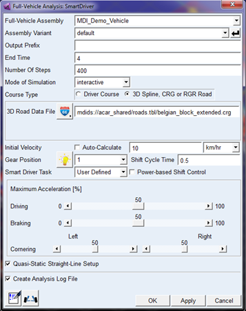
The spacing of the centerline points depends on the type of road:
1. Road files with extension .crg or .rgr:
For a CRG type of road (extension .crg) and RGR road with extension .rgr, the spacing in between the points is 1 meter.
2. Road files with extension .rdf:
3D Spline roads or rdf files referring to a .rgr file will take the points for the centerline as defined in the [DATA_POINTS] section.
Virtual Test Drive
The "VIRES Virtual Test Drive" application (https://vires.com) is used for the development and testing of advanced driver assistance and active safety systems, leading to solutions for automated driving.
This Adams Full Vehicle simulation dialog feature allows to prepare and develop an Adams Car full vehicle for use as a plant in the VTD simulation environment. First a full vehicle model needs to be assembled that can perform vehicle analysis maneuvers in real time.
The solver settings for the 'Adams as a Plant' simulation in VTD are important:
■The Fixed Time Step Solver needs to be used (with C++ Solver only).
■A basic interfacing frequency of 100 Hz is advised, implicating that the time step is 0.01 sec.
■By increasing the hratio factor, the model can run smaller solver steps.
■SMP (multi-threading) is supported.
No selection for the road is required because VTD will provide Adams with the road geometry on-line. Currently tire models can use the 'one point of contact' interface only.
In addition VTD will provide the Adams model of the steering, braking, throttle and gear (forward or backward) input; Adams will return the position and velocities of the vehicle body and wheels.
The model items and user subroutines required for the interface to VTD are part of the SDI Testrig Design Option. (Driving Machine State). When submitting a simulation for VTD, there is no need to change the Design Option, it will be set by the simulation submit macro.
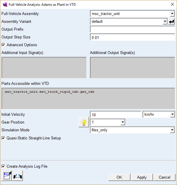
Two simulation modes are available:
■Interactive: Adams Car will prepare the model files and then start a simulation. In this mode the user has to start VTD manually before the Adams simulation is started. VTD should use the correct settings in order to interface with Adams Solver. VTD may run at a different platform than Adams Solver. The connection in between Adams and VTD is using the UPD RDB interface of VTD.
■Files_only: Adams Car will produce an FMU that can be imported into VTD.
Notes: | 1. In case of an interactive simulation and two different platforms are used for running Adams and VTD, one should take care that the UDP ports used for the RDB interface are not blocked. The ports used by this application are 48190, 48191, 48270 and 48271. 2. In case of an interactive simulation where the VTD application is to be accessed remotely from either Windows or Linux, common remote access software like RealVNC or MobaXterm are not supported. The one remote access software that does work is NoMachine freeware which is available for download at https://www.nomachine.com/download. |
Suspension Parameter Measurement Machine (SPMM) Analysis
You perform a SPMM analysis to measure Kinematic and Compliance (K&C) characteristics of vehicle due to suspension and steering system geometries, and compliances due to suspension springs, anti-roll bars, elastomeric bushes and component deformations.
SPMM applies known displacement, force and torque inputs and measure the quasi-statics suspension characteristics that are important to ride and handling.
By performing SPMM tests, you can make design changes to achieve performance targets and obtain important vehicle suspension parameters.
In Suspension Parameter Measurement Machine (SPMM) analysis, you can perform any or all of the following sub-events:
■Vertical Motion
■Roll Motion
■Steer Motion
■Compliance
■Aligning Torque
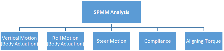
The __MDI_SPMM_TESTRIG test rig (Figure 16) is used for Suspension Parameter Measurement Machine (SPMM) analysis.
The __MDI_SPMM_TESTRIG actuates chassis part using motion in jounce, rebound and roll sub-events. The chassis part is fixed at the static configuration in the Steering, Compliance and Aligning torque sub-events. In Compliance and Aligning torque sub-events general forces are used to apply forces and moments at tire contact patch or at wheel center. In Steering sub-event steering wheel is actuated using rotational motion.
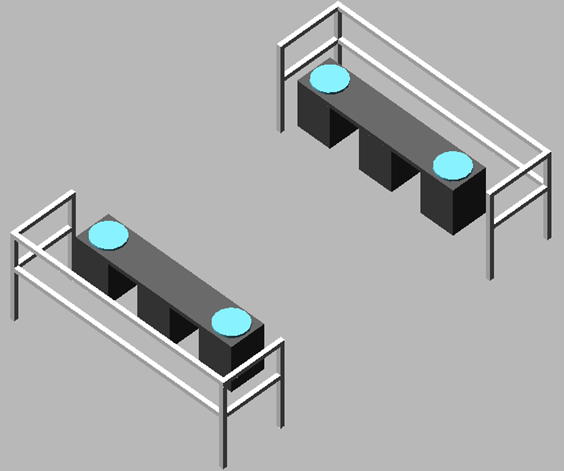
Figure 16 SPMM Testrig
To set up a Suspension Parameter Measurement Machine analysis:
1. From the Simulate menu, point to Full-Vehicle Analysis, point to Kinematic and Compliance, and then select Suspension Parameter Measurement Machine.
2. Enter the necessary parameters as explained in the dialog box help for Full-Vehicle Analysis: Suspension Parameter Measurement Machine.
3. Select OK.
Notes: | ■Before performing a SPMM analysis, you must specify several parameters about the vehicle in which you intend to use the suspension and steering subsystems. These parameters include the steering ratio, whether the suspension is front- or rear-wheel drive, and the braking ratio. To define vehicle parameters, see Full-Vehicle Analysis: Setup Parameters. ■The SPMM analysis first performs an equilibrium analysis, so the vehicle will settle on the suspension prior to the sub-events. Therefore the results may not directly comparable to suspension analysis results, since those are performed relative to design position by default. |
To view standard SPMM plots:
SPMM event creates plot configuration files (.plt) in your working directory with combination of output prefix and sub-events name (For example, '<output_prefix >_vertical_spmm.plt' for vertical motion sub-event). It also creates command file (.cmd) that can be used to import all the plt files. The plot configuration file includes pre-defined plots for the selected SPMM sub-events. The creation of plot configuration files per sub-event is as follows:
Sub-Event | Plot Configuration File |
|---|---|
Vertical | <output_prefix>_vertical_spmm.plt |
Roll | < output_prefix >_roll_spmm.plt |
Steer | < output_prefix >_steer_spmm.plt |
Compliance: | |
Longitudinal acceleration with brake torque off (contact_patch / wheel center) | < output_prefix >_long_<cp/wc>_accel_spmm.plt |
Longitudinal braking with brake torque on (contact_patch / wheel center) | < output_prefix >_long_<cp/wc>_brake_spmm.plt |
Lateral Parallel without trail | < output_prefix >_lat_par_spmm.plt |
Lateral Parallel with trail | < output_prefix >_lat_par_trail_<trail_value>_spmm.plt |
Lateral Opposite | < output_prefix >_lat_opp_spmm.plt |
Aligning: | |
Aligning Parallel | < output_prefix >_par_aligning_spmm.plt |
Aligning Opposite | < output_prefix >_opp_aligning_spmm.plt |
To view plots in the postprocessor, import "< output_prefix >_spmm_import.cmd".
To import each .plt file separately follow following steps:
1. Go to Postprocessing Window.
2. From the File menu, point to Import and then select Plot Config File
3. Enter the necessary parameters as explained in help for Creating Plots Using a Plot Configuration File.
4. Select OK.
To generate and view standard SPMM Report:
The report for SPMM event can be generated and displayed from event browser, you can right click on this event instance under event set, and select Review → Generate Report.
The SPMM report displays detailed information about vehicle K&C characteristics of vehicle.
When you simulate Suspension Parameter Measurement Machine event, the report file with extension <test_name>_spmm_rep.dat file will be generated in your working directory.
SPMM event has five different kinematic and compliance sub-events: Vertical Motion, Roll motion, Steer Motion, Compliance and Aligning Torque. If you uncheck any particular sub-event using "Active" toggle button, corresponding parameters of the events won't be displayed in the report. It will be displayed as "N/A".
The SPMM Report contains the parameters below reported at static condition:
Parameter | Information |
|---|---|
Date | Date and time of report generation |
Vehicle Assembly | Name of assembly used for SPMM analysis |
General Parameters: | |
Total Weight | Total weight of the vehicle. Summation of Front axle weight and Rear axle weight. |
Front Ground Reaction | Weight of the vehicle on front axle |
Rear Ground Reaction | Weight of the vehicle on rear axle |
Total Roll Inertia | Vehicle principal mass moments of inertia about vehicle center of mass and is oriented in GCS (X axis) |
Total Pitch Inertia | Vehicle principal mass moments of inertia about vehicle center of mass and is oriented in GCS (Y axis) |
Total Yaw Inertia | Vehicle principal mass moments of inertia about vehicle center of mass and is oriented in GCS (Z axis) |
Total Product Ixy | The cross products of inertia about vehicle center of mass and is oriented in GCS (X and Y axis) |
Total Product Ixz | The cross products of inertia about vehicle center of mass and is oriented in GCS (X and Z axis) |
Total Product Iyz | The cross products of inertia about vehicle center of mass and is oriented in GCS (Y and Z axis) |
Global C.G location | Location of Center of Gravity of vehicle at static condition from GCS |
Ground Plane Elevation | The movement of ground plane to bring it below the tires. |
C.G Height | The height of vehicle C.G. from ground plane |
Wheelbase | Distance between the front and rear wheel centers |
Average Track Width | The average of front and rear track width |
STATIC: | |
Static Toe (total / left / right)* | Toe specified in the alignment setting at static position. If adjuster force is defined and active in the subsystem, value in the report matches the alignment setting. |
Static Camber* | Camber specified in the alignment setting at static position. If adjuster force is defined and active in the subsystem, value in the report matches the alignment setting. |
Static Caster* | The angle in the side elevation between the steering axis (such as kingpin axis) and the vertical |
Kingpin Angle* | The angle in the front elevation between the steer axis (the kingpin axis) and the vehicle's vertical axis. It is positive when the steer axis is inclined upward and inward. |
Caster Trail* | The distance in side elevation between the point where the steering axis intersects the ground, and the center of tire contact. The trail (or offset) is considered positive when the intersection point is forward of the tire contact center and negative when it is rearward. |
Scrub Radius* | The distance from the point at the intersection of the kingpin axis and the ground plane to the line of intersection of the wheel and ground planes. Scrub radius is positive if the kingpin axis intersects the ground inboard of the wheel. |
Track Width* | The lateral distance between the centers of tire contact of the left and right wheels |
Roll Center Height* | The vertical distance of Roll center location from the ground plane. |
Roll Center lateral shift* | The lateral distance of Roll Center Location from the half-track. |
Wheel Center Rise | Difference in wheel center height, measured with respect to the body, between design and static equilibrium condition. |
Tire Rolling Radius | Static tire loaded radius |
BOUNCE TEST: | |
Wheel Rate* | The rate of change in normal tire force per unit change in vertical displacement of wheel center. OR The change of wheel load, at the center of tire contact, per unit vertical displacement of the sprung mass relative to the wheel. |
Spring Rate | The rate of change in spring length per unit displacement of spring displacement |
Spring Ratio | The rate of change in spring length per unit vertical displacement of the wheel center relative to the sprung mass |
Damper Ratio | The rate of change in damper length per unit vertical displacement of the wheel center relative to the sprung mass |
Spring Rate at Wheel | Calculated by taking the square of the spring ratio times the spring rate |
Bump Steer | Change in toe angle per unit vertical displacement of the wheel center. |
Bump Caster | Change in caster angle per unit vertical displacement of the wheel center |
Bump Camber | Change in camber angle per unit vertical displacement of the wheel center |
Longitudinal Wheel Center Recession | Change in horizontal displacement of the wheel center per unit vertical displacement of the wheel center |
Lateral Wheel Center Migration | Change in lateral displacement of the wheel center per unit vertical displacement of the wheel center |
ROLL TEST: | |
Wheel Rate in Roll | Change in normal tire force per unit change in vertical displacement |
Roll Stiffness | Resistance to chassis roll due to spring and/or anti roll bar. Roll stiffness is calculated as: Roll Stiffness = (( Σwheel rate * track2 ) / 4) * dtor |
Roll Steer (Per Degree)* | Change in toe angle per unit change in roll angle |
Roll Steer | Change in toe angle per unit change in vertical displacement of the wheel center |
Roll Camber w.r.t. Chassis (Per Degree) | Change in wheel inclination angle with respect to chassis per unit change in vehicle roll angle |
Roll Camber (Per Degree)* | Change in wheel inclination angle per unit change in vehicle roll angle |
Roll Camber | The rate of change in wheel inclination angle per unit change in vertical displacement of the wheel center |
Steering Wheel Torque vs Roll Angle | Change in steering wheel torque per unit change in roll angle |
STEER TEST: | |
Rack Travel @ steering input | Value of maximum rack travel reached at given steering input |
Max Steer Angle @steering input (Left Turn) | Maximum steer angle of inner and outer wheel at given steering input in left turn |
Max Steer Angle @steering input (Right Turn) | Maximum steer angle of inner and outer wheel at given steering input in right turn |
Full lock Angle @pvs_max_rack_disp (Left Turn) | Maximum steer angle of inner and outer wheel at given parameter pvs_max_rack_displacement in left turn. This will be displayed if rack travel reaches specified rack travel in parameter variable pvs_max_rack_displacement. |
Full lock Angle @pvs_max_rack_disp (Right Turn) | Maximum steer angle of inner and outer wheel at given parameter pvs_max_rack_displacement in right turn. This will be displayed if rack travel reaches specified rack travel in parameter variable pvs_max_rack_displacement. |
LONGITUDINAL COMPLIANCE TEST: | |
Brake Steer | Change in toe angle per unit change in longitudinal tire force at contact patch |
Traction Steer | Change in toe angle per unit longitudinal force at wheel center |
Contact Patch Braking Stiffness | Change in longitudinal tire force at contact patch per unit change in longitudinal tire displacement |
Wheel Center Longitudinal Stiffness | Change in longitudinal force at wheel center per unit change in longitudinal tire displacement |
Caster Compliance - Braking | Change in caster angle per unit longitudinal tire force at contact patch |
Caster Compliance - Traction | Change in caster angle per unit longitudinal force at wheel center |
LATERAL COMPLIANCE TEST - PARALLEL: | |
Lateral Force Steer Compliance* | Change in toe angle per unit lateral tire force at contact patch |
Lateral Force Camber Compliance* | Change in camber angle per unit lateral tire force at contact patch |
Wheel Center Lateral Stiffness* | Change in lateral tire force at contact patch per unit lateral tire displacement |
LATERAL COMPLIANCE TEST - OPPOSITE: | |
Lateral Force Steer Compliance* | Change in toe angle per unit lateral tire force at contact patch |
Lateral Force Camber Compliance* | Change in camber angle per unit lateral tire force at contact patch |
Wheel Center Lateral Stiffness* | Change in lateral tire force at contact patch per unit lateral tire displacement |
ALIGNING TORQUE TEST - PARALLEL: | |
Aligning Torque – Steer* | Change in steer angle per unit change in aligning torque on the wheel |
Aligning Torque - Camber* | Change in camber angle per unit change in aligning torque on the wheel |
ALIGNING TORQUE TEST - OPPOSITE: | |
Aligning Torque – Steer* | Change in steer angle per unit change in aligning torque on the wheel |
Aligning Torque - Camber* | Change in camber angle per unit change in aligning torque on the wheel |
* For detailed information refer to Running Analyses > Output of Suspension Analyses
To view SPMM Animations:
SPMM animation can be viewed as the continuous animation or a separate animation for each sub-events. By default, continuous animation is loaded when you select Review > Animation Controls… after the simulation. To view any sub-events animation, select the desired analysis in the analysis field of Animation Controls… dialog box.
To use flexible chassis with SPMM setup:
SPMM supports flexible chassis when created using following methods:
1. In Template Builder: Flexible chassis can be added into your body template (for example, 'rigid_chassis.tpl' or 'rigid_chassis_lt.tpl'). It can be done by making rigid ges_chassis part to a flexible ges_chassis_flex part and modifying bedplate location hardpoints (hp[lr]_bedplate_front_loc and hp[lr]_bedplate_rear_loc) to the appropriate interface node locations. If you create your own body template, you need to add the hardpoints and input communicators as defined in the acar_shared templates.
2. Subsystem/Assembly level (Standard Interface): Using Adjust > General Part > Rigid to Flex, swap existing rigid chassis to flex chassis and then modify the bedplate location hardpoints to the desired locations.
3. Assembly level (Standard Interface): Using File > Manage Assemblies > Replace Subsystem, replace the rigid chassis subsystem with a flexible chassis subsystem.
To use Engine On/Off and ARB On/Off options:
SPMM sub-events can be simulated with Engine On/Off and ARB On/Off option.
When Engine On/Off option is toggled to 'On' under the sub-events those events will run with additional events, that is, the first event will run with Engine 'On' and the second will run with Engine 'Off'. During this process steering boost force is deactivated.
Similarly, when ARB On/Off option is toggled to 'On' under the sub-events. All events will run with ARB 'On', followed by Engine On/Off if that option is selected. After that, only those events will run with ARB 'Off', followed by Engine On/Off if that option is selected. During this process ARB droplink joint/bushing (whichever is communicated and active) is deactivated.
For Engine On/Off and ARB On/Off to work, you need to add following output communicator to respective templates as shown in below table.
Option | Template Role | Communicator Matching Name | Entity | Type |
|---|---|---|---|---|
Engine On/Off | Steering | steering_assist_force | force | Single |
ARB On/Off | Antirollbar/Suspension (if ARB is modelled as part of suspension) | arb_droplink_joint / arb_droplink_bushing | Joint / bushing | Left/Right |
Kinematic and Compliance (KnC) Static/Dynamic Analysis
KnC Static and Dynamic analysis is the derivative of SPMM analysis. In KnC analysis vertical and roll motion actuation are carried out by actuating Wheel part instead of body as in SPMM as shown in following chart.
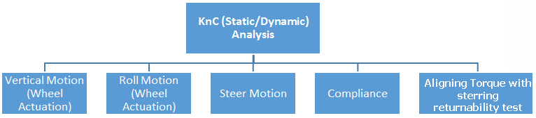
The __MDI_SPMM_TESTRIG test rig (Figure 17) with some graphical changes is used for KnC analysis.
The __MDI_SPMM_TESTRIG actuates wheel part using motion in jounce, rebound and roll sub-events. The chassis part is fixed at the static configuration in the Vertical, Roll, Steering, Compliance and Aligning torque sub-events. In Compliance and Aligning torque sub-events general forces are used to apply forces and moments at tire contact patch or at wheel center. In Steering sub-event steering wheel is actuated using rotational motion.
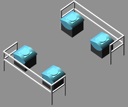
Figure 17 KnC Testrig
Difference between KnC Static and Dynamic analysis:
KnC Static | KnC Dynamic |
|---|---|
The tire forces are set to zero after initial static analysis (SVC). The wheel parts are connected to pad using spherical joint and bushing has a stiffness to resist aligning moment. | No Changes in model after initial static analysis |
The subevents except steering returnability will be performed as quasi-static simulation. The steering returnability subevent will be performed as transient simulation. | All subevents are performed as transient simulation. |
To set up a Kinematic and Compliance analysis:
1. From the Simulate menu, point to Full-Vehicle Analysis, point to Kinematic and Compliance, and then select KnC (Static) or KnC (Dynamic).
2. Enter the necessary parameters as explained in the dialog box help for Full-Vehicle Analysis: Kinematic and Compliance (Static / Dynamic).
3. Select OK.
Note: | Before performing a KnC analysis, you must specify several parameters about the vehicle in which you intend to use the suspension and steering subsystems. These parameters include the steering ratio, whether or not the suspension is front- or rear-wheel drive, and the braking ratio. To define vehicle parameters, see Full-Vehicle Analysis: Setup Parameters. |
To view standard KnC plots
KnC event creates plot configuration files (.plt) in your working directory with combination of output prefix and sub-events name (for example, '<output_prefix >_vertical_kcse.plt' for static vertical motion sub-event and '<output_prefix >_vertical_dkcse.plt' for dynamic vertical motion sub-event). It also creates command file (.cmd) that can be used to import all the plt files. The plot configuration file includes pre-defined plots for the selected KnC sub-events. The creation of plot configuration files per sub-event is as follows:
Sub-Event | Plot Configuration File |
|---|---|
Vertical | <output_prefix>_vertical_[d]kcse.plt |
Roll | < output_prefix >_roll_[d]kcse.plt |
Steer | < output_prefix >_steer_[d]kcse.plt |
Compliance: | |
Longitudinal acceleration with brake torque off depending upon powertrain role. For front, rear and any role, only front, rear and all wheel brakes are released respectively. (contact_patch / wheel center) | < output_prefix >_long_<cp/wc>_accel_d]kcse.plt |
Longitudinal braking with brake torque on (contact_patch / wheel center) | < output_prefix >_long_<cp/wc>_brake_ [d]kcse.plt |
Lateral Parallel without trail | < output_prefix >_lat_par _[d]kcse.plt |
Lateral Parallel with trail | < output_prefix >_lat_par_trail_<trail_value>_[d]kcse.plt |
Lateral Opposite | < output_prefix >_lat_opp_compliance_[d]kcse.plt |
Aligning: | |
Aligning Parallel | < output_prefix >_par_aligning_[d]kcse.plt |
Aligning Opposite | < output_prefix >_opp_aligning_[d]kcse.plt |
Report
The report for Kinematic and Compliance event can be generated and displayed from event browser, you can right click on this event instance under event set, and select Review → Generate Report.
When you simulate Kinematic and Compliance event, report file with extension <test_name>_[d]kcse_rep.dat file will be generated in your working directory.
Kinematic and Compliance event has five different kinematic and compliance sub-events: Vertical Motion, Roll motion, Steer Motion, Compliance and Aligning Torque. If you uncheck any particular sub-event using "Active" toggle button, corresponding parameters of the events won't be displayed in the report. It will be displayed as "N/A".
For details on report generation and its parameters descriptions, Animations, flexible chassis and Engine On/Off and ARB On/Off refer respective sections under Suspension Parameter Measurement Machine (SPMM) Analysis.
Static Vehicle Characteristics (SVC) Analysis
Static Vehicle Characteristics (SVC) refers to a set of Adams utility subroutines (CONSUB) which compute Static Vehicle Characteristics (SVC) for automobile or light truck suspensions at static equilibrium. For a full vehicle, SVC calculates characteristics for the front and rear suspension as well as general vehicle characteristics such as ground reactions and mass properties. For more details, see Static Vehicle Characteristics (SVC) help.
A CONSUB controls this analysis. For more information on CONSUB, see Welcome to Adams Solver Subroutines.
To set up a Static Vehicle Characteristics (SVC) analysis:
1. From the Simulate menu, point to Full-Vehicle Analysis, point to Static and Quasi-Static Maneuvers and then select Static Vehicle Characteristics.
2. Press F1 and then follow the instructions in the dialog box help for Full-Vehicle Analysis: Static Vehicle Characteristics.
3. Select OK.
SmartDriver Setting Template
The SmartDriver Setting Template file (basically an .xml event file without events) is used to set default values for Event files. The default values are used when:
■converting .dcf format Event files to .xml format Event files.
■creating new Event files using the Event Builder.
You can use environment variable MSC_SD_DEFAULT_XML to set the path to a custom SmartDriver Setting Template file (.smartdriver.xml). If MSC_SD_DEFAULT_XML is not set, the SmartDriver Setting Template file path search order is as follows:
1. Home directory ($HOME\.smartdriver.xml)
2. \<Adams Installation>\<platform>\ ($topdir\$MDI_CPU\.smartdriver.xml)